19. Phased Arrays with Phaser

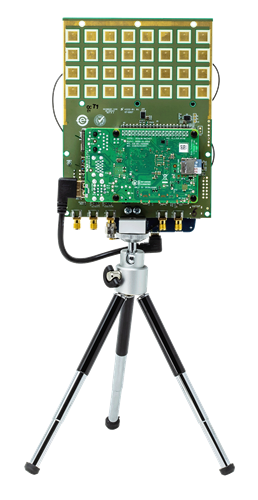
In this chapter we use the Analog Devices Phaser, (a.k.a. CN0566 or ADALM-PHASER) which is an 8-channel low-cost phased array SDR that combines a PlutoSDR, Raspberry Pi, and ADAR1000 beamformers, designed to operate around 10.25 GHz. We will cover the setup and calibration steps, and then go through some beamforming examples in Python. For those that do not have a Phaser, we have included screenshots and animations of what the user would see.

Hardware Overview

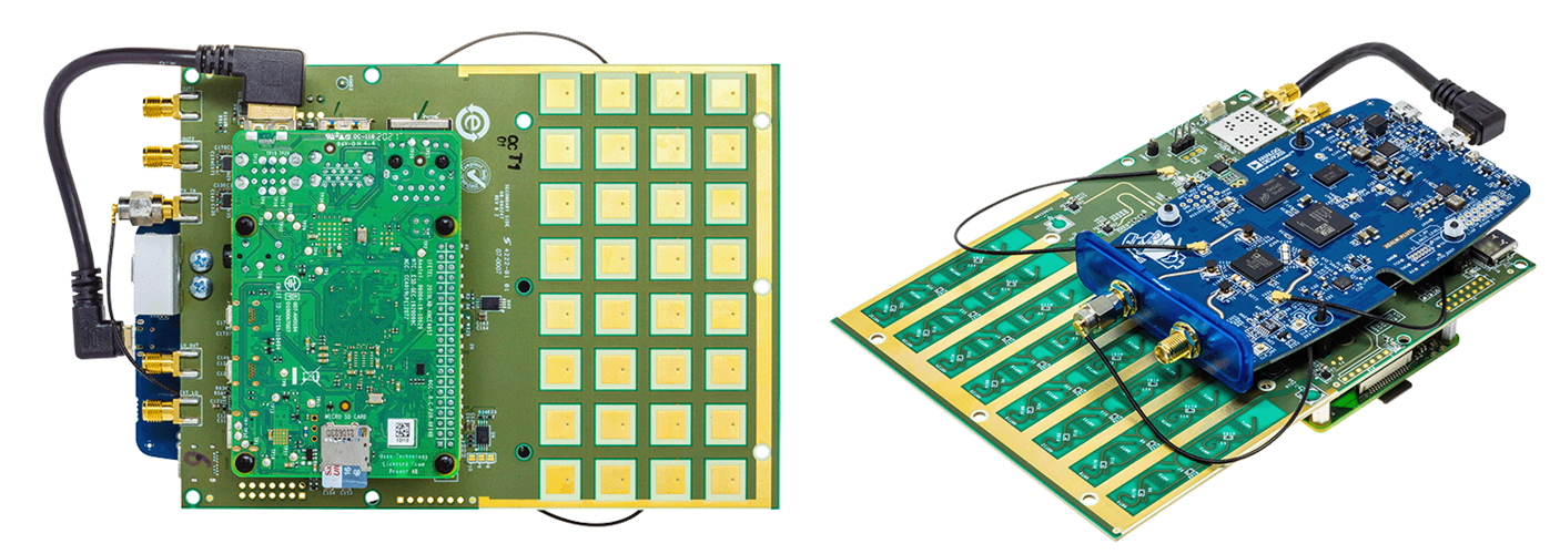
The Phaser is a single board containing the phased array and a bunch of other components, with a Raspberry Pi plugged in on one side and a Pluto mounted to the other side. The high-level block diagram is shown below. Some items to note:

1. Even though it looks like a 32-element 2d array, it’s really an 8-element 1d array

2. Both receive channels on the Pluto are used (the second channel uses a u.FL connector)

3. The LO onboard is used to downconvert the received signal from around 10.25 GHz to around 2 GHz, so that the Pluto can receive it

4. Each ADAR1000 has four phase shifters with adjustable gain, and all four channels are summed together before being sent to the Pluto

5. The Phaser essentially contains two “subarrays” which each subarray containing four channels

6. Not shown below are GPIO and serial signals from the Raspberry Pi used to control various components on the Phaser

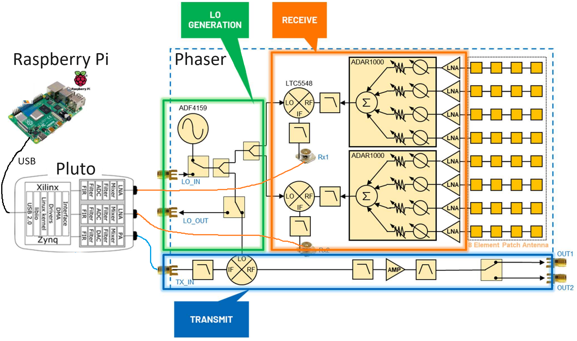
For now let’s ignore the transmit side of the Phaser, as in this chapter we will only be using the HB100 device as a test transmitter. The ADF4159 is a frequency synthesizer that produces a tone up to 13 GHz in frequency, what we call the local oscillator or LO. This LO is fed into a mixer, the LTC5548, which is able to do upconversion or downconversion, although we’ll be using it for downconversion. For downconversion it takes in the LO as well as a signal anywhere from 2 - 14 GHz, and multiplies the two together which performs a frequency shift. The resulting downconverted signal can be anywhere from DC to 6 GHz, although we are going to target around 2 GHz. The ADAR1000 is a 4-channel analog beamformer, so the Phaser utilizes two of them. An analog beamformer has independently adjustable phase shifters and gain for each channel, allowing each channel to be time-delayed and attenuated before being summed together in the analog domain (resulting in a single channel). On the Phaser, each ADAR1000 outputs a signal which gets downconverted and then received by the Pluto. Using the Raspberry Pi we can control the phase and gain of all eight channels in real-time, to perform beamforming. We also have the option to do two-channel digital beamforming/array processing, discussed in the next chapter.

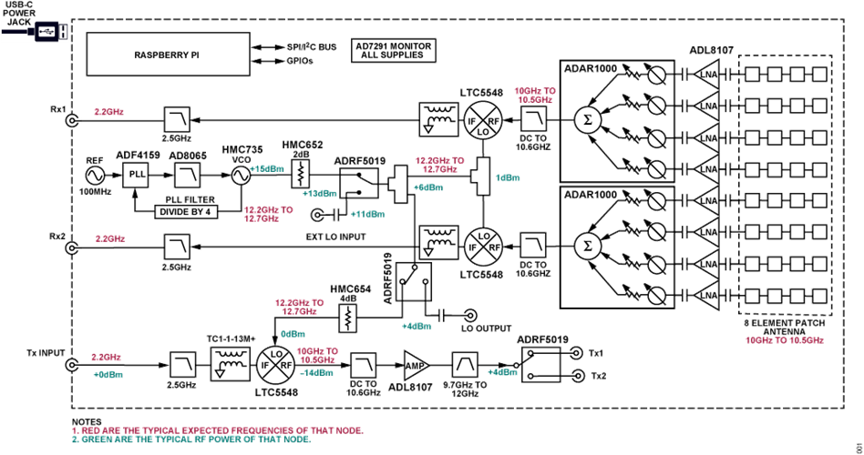
For those interested, a slightly more detailed block diagram is provided below.

SD Card Preparation

We will assume you are using the Raspberry Pi onboard the Phaser (directly, with a monitor/keyboard/mouse). This simplifies setup, as Analog Devices publishes a pre-built SD card image with all the necessary drivers and software. You can download the SD card image and find SD imaging instructions here. The image is based on Raspberry Pi OS and includes all the software you’ll need already installed.

Hardware Preparation

1. Connect Pluto’s CENTER micro-USB port to Raspberry Pi

2. Optionally, carefully thread the tripod into the tripod mount

3. We will assume you’re using an HDMI display, USB keyboard, and USB mouse connected to the Raspberry pi

4. Power the Pi and Phaser board through the type-C port of the Phaser (CN0566), i.e. do NOT connect a supply to the Raspberry Pi’s USB C

Software Install

Once you have booted into the Raspberry Pi using the pre-build image, using the default user/pass analog/analog, it is recommended to run the following steps:

wget https://github.com/mthoren-adi/rpi_setup_stuff/raw/main/phaser/phaser_sdcard_setup.sh
sudo chmod +x phaser_sdcard_setup.sh
./phaser_sdcard_setup.sh
sudo reboot

sudo raspi-config

For more assistance setting up the Phaser, reference the Phaser wiki quickstart page.

HB100 Setup

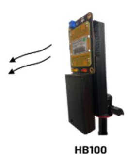
The HB100 that comes with the Phaser is a low-cost Doppler radar module that we will be using as a test transmitter, as it transmits a continuous tone around 10 GHz. It runs off 2 AA batteries or a 3V benchtop supply, and when it’s on it will have a solid red LED.

Because the HB100 is low-cost and uses cheap RF components, its transmit frequency varies from unit to unit, over hundreds of MHz, which is a range that is greater than the highest bandwidth we can receive using the Pluto (56 MHz). So to make sure we are tuning our Pluto and downconverter in a manner that will always receive the HB100 signal, we must determine the HB100’s transmit frequency. This is done using an example app from Analog Devices, which performs a frequency sweep and calculates FFTs while looking for a spike. Make sure your HB100 is on and in the general vicinity of the Phaser, and then run the utility with:

cd ~/pyadi-iio/examples/phaser
python phaser_find_hb100.py

It should create a file called hb100_freq_val.pkl in the same directory. This file contains the HB100 transmit frequency in Hz (pickled, so not viewable in plaintext) which we will use in the next step.

Calibration

Lastly, we need to calibrate the phased array. This requires holding the HB100 at the array’s boresight (0 degrees). The side of the HB100 with the barcode is the side that transmits the signal, so that face should be held a few feet away from the Phaser, right in-front and centered to it, and then pointed straight at the Phaser. In the next step you can experiment with different angles and orientations, but for now let’s run the calibration utility:

python phaser_examples.py cal

This will create two more pickle files: phase_cal_val.pkl and gain_cal_val.pkl, in the same directory. Each one contains an array of 8 numbers corresponding to the phase and gain tweaks needed to calibrate each channel. These values are unique to each Phaser, as they can very during manufacturing. Subsequent runs of this utility will lead to slightly different values which is normal.

Pre-built Example App

Now that we have calibrated our Phaser and found the HB100 frequency, we can run the example app that Analog Devices provides.

python phaser_gui.py

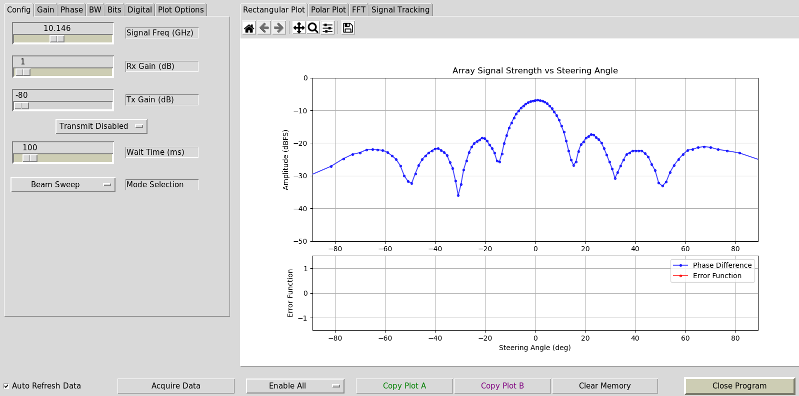
If you check the “Auto Refresh Data” checkbox in the bottom-left it should begin running. You should see something similar to the following when holding the HB100 in the Phaser’s boresight.

Phaser in Python

We will now dive into the hands-on Python portion. For those who don’t have a Phaser, screenshots and animations are provided.

Initializing Phaser and Pluto

The following Python code sets up our Phaser and Pluto. By this point you should have already run the calibration steps, which produce three pickle files. Make sure you are running the Python script below from within the same directory as these pickle files.

There are a lot of settings to deal with, so it’s OK if you don’t absorb the entire code snippet below, just note that we are using a sample rate of 30 MHz, manual gain which we set very low, we set all of the element gains to the same value, and point the array towards boresight (0 degrees).

import time
import sys
import matplotlib.pyplot as plt
import numpy as np
import pickle
from adi import ad9361
from adi.cn0566 import CN0566

phase_cal = pickle.load(open("phase_cal_val.pkl", "rb"))
gain_cal = pickle.load(open("gain_cal_val.pkl", "rb"))
signal_freq = pickle.load(open("hb100_freq_val.pkl", "rb"))
d = 0.014  # element to element spacing of the antenna

phaser = CN0566(uri="ip:localhost")
sdr = ad9361(uri="ip:192.168.2.1")
phaser.sdr = sdr
print("PlutoSDR and CN0566 connected!")

time.sleep(0.5) # recommended by Analog Devices

phaser.configure(device_mode="rx")

# Set all antenna elements to half scale - a typical HB100 will have plenty of signal power.
gain = 64 # 64 is about half scale
for i in range(8):
    phaser.set_chan_gain(i, gain, apply_cal=False)

# Aim the beam at boresight (zero degrees)
phaser.set_beam_phase_diff(0.0)

# Misc SDR settings, not super critical to understand
sdr._ctrl.debug_attrs["adi,frequency-division-duplex-mode-enable"].value = "1"
sdr._ctrl.debug_attrs["adi,ensm-enable-txnrx-control-enable"].value = "0" # Disable pin control so spi can move the states
sdr._ctrl.debug_attrs["initialize"].value = "1"
sdr.rx_enabled_channels = [0, 1] # enable Rx1 and Rx2
sdr._rxadc.set_kernel_buffers_count(1) # No stale buffers to flush
sdr.tx_hardwaregain_chan0 = int(-80) # Make sure the Tx channels are attenuated (or off)
sdr.tx_hardwaregain_chan1 = int(-80)

# These settings are basic PlutoSDR settings we have seen before
sample_rate = 30e6
sdr.sample_rate = int(sample_rate)
sdr.rx_buffer_size = int(1024)  # samples per buffer
sdr.rx_rf_bandwidth = int(10e6)  # analog filter bandwidth

# Manually gain (no automatic gain control) so that we can sweep angle and see peaks/nulls
sdr.gain_control_mode_chan0 = "manual"
sdr.gain_control_mode_chan1 = "manual"
sdr.rx_hardwaregain_chan0 = 10 # dB, 0 is the lowest gain.  the HB100 is pretty loud
sdr.rx_hardwaregain_chan1 = 10 # dB

sdr.rx_lo = int(2.2e9) # The Pluto will tune to this freq

# Set the Phaser's PLL (the ADF4159 onboard) to downconvert the HB100 to 2.2 GHz plus a small offset
offset = 1000000 # add a small arbitrary offset just so we're not right at 0 Hz where there's a DC spike
phaser.lo = int(signal_freq + sdr.rx_lo - offset)

Receiving Samples from the Pluto

At this point the Phaser and Pluto are configured and ready to go. We can now start receiving data from the Pluto. Let’s grab a single batch of 1024 samples, then take the FFT of each of the two channels.

# Grab some samples (whatever we set rx_buffer_size to), remember we are receiving on 2 channels at the same time
data = sdr.rx()

# Take FFT
PSD0 = 10*np.log10(np.abs(np.fft.fftshift(np.fft.fft(data[0])))**2)
PSD1 = 10*np.log10(np.abs(np.fft.fftshift(np.fft.fft(data[1])))**2)
f = np.linspace(-sample_rate/2, sample_rate/2, len(data[0]))

# Time plot helps us check that we see the HB100 and that we're not saturated (ie gain isnt too high)
plt.subplot(2, 1, 1)
plt.plot(data[0].real) # Only plot real part
plt.plot(data[1].real)
plt.xlabel("Data Point")
plt.ylabel("ADC output")

# PSDs show where the HB100 is and verify both channels are working
plt.subplot(2, 1, 2)
plt.plot(f/1e6, PSD0)
plt.plot(f/1e6, PSD1)
plt.xlabel("Frequency [MHz]")
plt.ylabel("Signal Strength [dB]")
plt.tight_layout()
plt.show()

What you see at this point will depend if your HB100 is on and where it’s pointing. If you hold it a few feet from the Phaser and point it towards the center, you should see something like this:

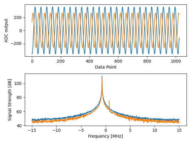
Note the strong spike near 0 Hz, the 2nd shorter spike is simply an artifact that can be ignored, since it’s around 40 dB down. The top plot, showing the time domain, displays the real part of the two channels, so the relative amplitude between the two will vary slightly depending on where you hold the HB100.

Performing Beamforming

Next, let’s actually sweep the phase! In the following code we sweep the phase from negative 180 to positive 180 degrees, at a 2 degree step. Note that this is not the angle the beamformer points; it’s the phase difference between adjacent channels. We must calculate the angle of arrival corresponding to each phase step, using knowledge of the speed of light, the RF frequency of the received signal, and the Phaser’s element spacing. The phase difference between adjacent elements is given by:

where is the angle of arrival of the signal with respect to boresight, is the antenna spacing in meters, and is the wavelength of the signal. Using the formula for wavelength and solving for we get:

You’ll see this when we calculate steer_angle below:

powers = [] # main DOA result
angle_of_arrivals = []
for phase in np.arange(-180, 180, 2): # sweep over angle
    print(phase)
    # set phase difference between the adjacent channels of devices
    for i in range(8):
        channel_phase = (phase * i + phase_cal[i]) % 360.0 # Analog Devices had this forced to be a multiple of phase_step_size (2.8125 or 360/2**6bits) but it doesn't seem nessesary
        phaser.elements.get(i + 1).rx_phase = channel_phase
    phaser.latch_rx_settings() # apply settings

    steer_angle = np.degrees(np.arcsin(max(min(1, (3e8 * np.radians(phase)) / (2 * np.pi * signal_freq * phaser.element_spacing)), -1))) # arcsin argument must be between 1 and -1, or numpy will throw a warning
    # If you're looking at the array side of Phaser (32 squares) then add a *-1 to steer_angle
    angle_of_arrivals.append(steer_angle)
    data = phaser.sdr.rx() # receive a batch of samples
    data_sum = data[0] + data[1] # sum the two subarrays (within each subarray the 4 channels have already been summed)
    power_dB = 10*np.log10(np.sum(np.abs(data_sum)**2))
    powers.append(power_dB)
    # in addition to just taking the power in the signal, we could also do the FFT then grab the value of the max bin, effectively filtering out noise, results came out almost exactly the same in my tests
    #PSD = 10*np.log10(np.abs(np.fft.fft(data_sum * np.blackman(len(data_sum))))**2) # in dB

powers -= np.max(powers) # normalize so max is at 0 dB

plt.plot(angle_of_arrivals, powers, '.-')
plt.xlabel("Angle of Arrival")
plt.ylabel("Magnitude [dB]")
plt.show()

For each phase value (remember, this is the phase between adjacent elements) we set the phase shifters, after adding in the phase calibration values and forcing the degrees to be between 0 and 360. We then grab one batch of samples with rx(), sum the two channels, then calculate the power in the signal. We then plot power over angle of arrival. The result should look something like this:

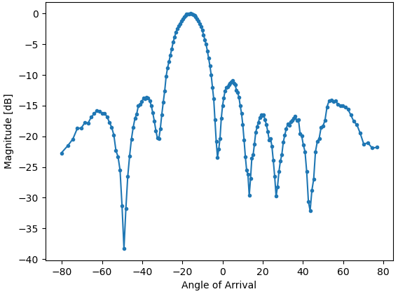
In this example the HB100 was held slightly to the side of boresight.

If you want a polar plot you can instead using the following:

# Polar plot
fig, ax = plt.subplots(subplot_kw={'projection': 'polar'})
ax.plot(np.deg2rad(angle_of_arrivals), powers) # x axis in radians
ax.set_rticks([-40, -30, -20, -10, 0])  # Less radial ticks
ax.set_thetamin(np.min(angle_of_arrivals)) # in degrees
ax.set_thetamax(np.max(angle_of_arrivals))
ax.set_theta_direction(-1) # increase clockwise
ax.set_theta_zero_location('N') # make 0 degrees point up
ax.grid(True)
plt.show()

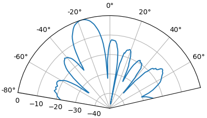
By taking the max we can estimate the direction of arrival of the signal!

Real-time and with Spatial Tapering

Now let’s take a moment to talk about spatial tapering. So far we have left the gain adjustments of each channel to equal values, so that all eight channels get summed equally. Just like we applied a window before taking an FFT, we can apply a window in the spatial domain by applying weights to these eight channels. We’ll use the exact same windowing functions like Hanning, Hamming, etc. Let’s also tweak the code to run in real-time so that it’s a little more fun:

plt.ion() # needed for real-time view
print("Starting, use control-c to stop")
try:
    while True:
        powers = [] # main DOA result
        angle_of_arrivals = []
        for phase in np.arange(-180, 180, 6): # sweep over angle
            # set phase difference between the adjacent channels of devices
            for i in range(8):
                channel_phase = (phase * i + phase_cal[i]) % 360.0 # Analog Devices had this forced to be a multiple of phase_step_size (2.8125 or 360/2**6bits) but it doesn't seem nessesary
                phaser.elements.get(i + 1).rx_phase = channel_phase

            # set gains, incl the gain_cal, which can be used to apply a taper.  try out each one!
            gain_list = [127] * 8 # rectangular window          [127, 127, 127, 127, 127, 127, 127, 127]
            #gain_list = np.rint(np.hamming(8) * 127)         # [ 10,  32,  82, 121, 121,  82,  32,  10]
            #gain_list = np.rint(np.hanning(10)[1:-1] * 127)  # [ 15,  52,  95, 123, 123,  95,  52,  15]
            #gain_list = np.rint(np.blackman(10)[1:-1] * 127) # [  6,  33,  80, 121, 121,  80,  33,   6]
            #gain_list = np.rint(np.bartlett(10)[1:-1] * 127) # [ 28,  56,  85, 113, 113,  85,  56,  28]
            for i in range(8):
                channel_gain = int(gain_list[i] * gain_cal[i])
                phaser.elements.get(i + 1).rx_gain = channel_gain

            phaser.latch_rx_settings() # apply settings

            steer_angle = np.degrees(np.arcsin(max(min(1, (3e8 * np.radians(phase)) / (2 * np.pi * signal_freq * phaser.element_spacing)), -1))) # arcsin argument must be between 1 and -1, or numpy will throw a warning
            angle_of_arrivals.append(steer_angle)
            data = phaser.sdr.rx() # receive a batch of samples
            data_sum = data[0] + data[1] # sum the two subarrays (within each subarray the 4 channels have already been summed)
            power_dB = 10*np.log10(np.sum(np.abs(data_sum)**2))
            powers.append(power_dB)

        powers -= np.max(powers) # normalize so max is at 0 dB

        # Real-time view
        plt.plot(angle_of_arrivals, powers, '.-')
        plt.xlabel("Angle of Arrival")
        plt.ylabel("Magnitude [dB]")
        plt.draw()
        plt.pause(0.001)
        plt.clf()

except KeyboardInterrupt:
    sys.exit() # quit python

You should see a real-time version of the previous exercise. Try switching which gain_list is used, to play around with the different windows. Here is an example of the Rectangular window (i.e., no windowing function):

and here is an example of the Hamming window:

Note the lack of sidelobes for Hamming. In fact, every window aside from Rectangular will greatly reduce the sidelobes, but in return the main lobe will be a little wider.

Monopulse Tracking

Up until this point we have been performing individual sweeps in order to find the angle of arrival of a test transmitter (the HB100). But lets say we wish to continuously receive a communications or radar signal, that may be moving an causing the angle of arrival to change over time. We refer to this process as tracking, and it assumes we already have a rough estimate of the angle of arrival (i.e., the initial sweep has identified a signal of interest). We will use monopulse tracking to adaptively update the weights in order to keep the main lobe pointed at the signal over time, although note that there are other methods of tracking besides monopulse.

Invented in 1943 by Robert Page at the Naval Research Laboratory (NRL), the basic concept of monopulse tracking is to use two beams, both slightly offset from the current angle of arrival (or at least our estimate of it), but on different sides as shown in the diagram below.

We then take both the sum and difference (a.k.a. delta) of these two beams digitally, which means we must use two digital channels of the Phaser, making this a hybrid array approach (although you could certainly do the sum and difference in analog with custom hardware). The sum beam will equate to a beam centered at the current angle of arrival estimate, as shown above, which means this beam can be used for demod/decoding the signal of interest. The delta beam, as we will call it, is harder to visualize, but it will have a null at the angle of arrival estimate. We can use the ratio between the sum beam and delta beam (refered to as the error) to perform our tracking. This process is best explained with a short Python snippet; recall that the rx() function returns a batch of samples from both channels, so in the code below data[0] is the first channel of the Pluto (first set of four Phaser elements) and data[1] is the second channel (second set of four elements). In order to create two beams, we will steer each of the two sets separately. We can calculate the sum, delta, and error as follows:

data = phaser.sdr.rx()
sum_beam = data[0] + data[1]
delta_beam = data[0] - data[1]
error = np.mean(np.real(delta_beam / sum_beam))

The sign of the error tells us which direction the signal is actually coming from, and the magnitude tells us how far off we are from the signal. We can then use this information to update the angle of arrival estimate and weights. By repeating this process in real-time we can track the signal.

Now jumping into the full Python example, we will start by copying the code we used earlier to perform a 180 degree sweep. The only code we will add is to pull out the phase at which the received power was maximum:

# Sweep phase once to get initial estimate for AOA, using code above
# ...
current_phase = phase_angles[np.argmax(powers)]
print("max_phase:", current_phase)

Next we will create two beams, we will start by trying 5 degrees lower and 5 degrees higher than the current estimate, although note that this is in units of phase, we haven’t converted to steering angle, although they are similar. The following code is essentially two copies of the code we used earlier to set the phase shifters of each channel, except we use the first 4 elements for the lower beam and last 4 elements for upper beam:

# Now we create the two beams on either side of our current estimate
phase_offset = np.radians(5) # TRY TWEAKING THIS - specify offset from center in degrees
phase_lower = current_phase - phase_offset
phase_upper = current_phase + phase_offset
# first 4 elements will be used for lower beam
for i in range(0, 4):
   channel_phase = (phase_lower * i + phase_cal[i]) % 360.0
   phaser.elements.get(i + 1).rx_phase = channel_phase
# last 4 elements will be used for upper beam
for i in range(4, 8):
   channel_phase = (phase_upper * i + phase_cal[i]) % 360.0
   phaser.elements.get(i + 1).rx_phase = channel_phase
phaser.latch_rx_settings() # apply settings

Before doing the actual tracking, lets test the above by keeping the beam weights constant and moving the HB100 left and right (after it finishes initializing to find the starting angle):

print("START MOVING THE HB100 A LITTLE LEFT AND RIGHT")
error_log = []
for i in range(1000):
   data = phaser.sdr.rx() # receive a batch of samples
   sum_beam = data[0] + data[1]
   delta_beam = data[0] - data[1]
   error = np.mean(np.real(delta_beam / sum_beam))
   error_log.append(error)
   print(error)
   time.sleep(0.01)

plt.plot(error_log)
plt.plot([0,len(error_log)], [0,0], 'r--')
plt.xlabel("Time")
plt.ylabel("Error")
plt.show()

What’s happening in this example is I’m moving the HB100 around. I start by holding it in a steady position while the 180 degree sweep happens, then after it’s done I move it a little to the right, and wiggle it around, then I move it to the left of where I started and wiggle it around. Then around time = 400 in the plot I move it back to the other side and hold it there for a moment, before waving it around one more time. The take-away is that the further the HB100 gets from the starting angle, the higher the error, and the sign of the error tells us which side the HB100 is on relative to the starting angle.

Now lets use the error value to update the weights. We will get rid of the previous for loop, and make a new for loop around the entire process. For the sake of clarity we have the entire code example below, except for the initial part where we did the 180 degree sweep:

# Sweep phase once to get initial estimate for AOA
# ...
current_phase = phase_angles[np.argmax(powers)]
print("max_phase:", current_phase)

# Now we'll actually update the current_phase based on the error
print("START MOVING THE HB100 A LITTLE LEFT AND RIGHT")
phase_log = []
error_log = []
for ii in range(500):
   # Now we create the two beams on either side of our current estimate, using the specified offset
   phase_offset = np.radians(5)
   phase_lower = current_phase - phase_offset
   phase_upper = current_phase + phase_offset
   # first 4 elements will be used for lower beam
   for i in range(0, 4):
         channel_phase = (phase_lower * i + phase_cal[i]) % 360.0
         phaser.elements.get(i + 1).rx_phase = channel_phase
   # last 4 elements will be used for upper beam
   for i in range(4, 8):
         channel_phase = (phase_upper * i + phase_cal[i]) % 360.0
         phaser.elements.get(i + 1).rx_phase = channel_phase
   phaser.latch_rx_settings() # apply settings

   data = phaser.sdr.rx() # receive a batch of samples
   sum_beam = data[0] + data[1]
   delta_beam = data[0] - data[1]
   error = np.mean(np.real(delta_beam / sum_beam))
   error_log.append(error)
   print(error)

   # Update our estimated angle of arrival based on error
   current_phase += -10 * error # was manually tweaked until it seemed to track at a nice speed
   steer_angle = np.degrees(np.arcsin(max(min(1, (3e8 * np.radians(current_phase)) / (2 * np.pi * signal_freq * phaser.element_spacing)), -1)))
   phase_log.append(steer_angle) # looks nicer to plot steer angle instead of straight phase

   time.sleep(0.01)

fig, [ax0, ax1] = plt.subplots(2, 1, figsize=(8, 10))

ax0.plot(phase_log)
ax0.plot([0,len(phase_log)], [0,0], 'r--')
ax0.set_xlabel("Time")
ax0.set_ylabel("Phase Estimate [degrees]")

ax1.plot(error_log)
ax1.plot([0,len(error_log)], [0,0], 'r--')
ax1.set_xlabel("Time")
ax1.set_ylabel("Error")

plt.show()

You can see the error is essentially the derivative of the phase estimate; because we’re performing successful tracking, the phase estimate is more or less the actual angle of arrival. It’s not clear looking only at these plots, but when there is a sudden movement, it takes the system a small fraction of a second to adjust and catch up. The goal is for the change in angle of arrival to never be so quick that the signal arrives beyond the main lobes of the two beams.

It is a lot easier to visualize the process when the array is only 1D, but practical use-cases of monopulse tracking are almost always 2D (using a 2D/planar array instead of a linear array like the Phaser). For the 2D case, there are four beams created instead of two, and after process there is a single sum beam and four delta beams used to steer in both dimensions.

Radar with Phaser

Coming soon!

Conclusion

The entire code used to generate the figures in this chapter is available on the textbook’s GitHub page.