16. DOA & Beamforming¶

We zullen in dit hoofdstuk het gaan hebben over de concepten van bundelvorming (eng: beamforming), direction-of-arrival (DOA) (Nederlands: aankomstrichting) en phased arrays. Met behulp van Python simulatievoorbeelden worden Technieken zoals Capon en MUSIC besproken. We behandelen beamforming vs. DOA en twee verschillende soorten phased arrays (passief en actief). N.B. Dit hoofdstuk wordt momenteel vertaald en kan nog fouten bevatten.

16.1. Overzicht en termen¶

Een phased array, ook wel een elektronisch gestuurd array genoemd, is een array van antennes die aan de zend- of ontvangstkant kan worden gebruikt om (elektronische) bundels op een bepaalde richting op te focussen. Deze techniek wordt gebruikt in communicatie- en radartoepassingen.

Phased arrays kun je grofweg in drie categorieën indelen:

Passive electronically scanned array (PESA), beter bekend als een analoge of traditionele phased array. Hierbij worden analoge faseverschuivers gebruikt om de bundelrichting aan te passen. Bij de ontvanger worden alle elementen na een faseverschuiving (en eventueel versterking) opgeteld en met een mixer naar de basisband geschoven om te verwerken. Bij de zender gebeurt het tegenovergestelde; een enkel digitaal signaal wordt analoog gemaakt waarna meerdere faseverschuivers en versterkers worden gebruikt om het signaal voor elke antenne te produceren.
Active electronically scanned array (AESA), beter bekend als een volledig digitale array. Hier heeft elk element zijn eigen RF-componenten en het richten van de bundel gebeurt dan volledig digitaal. Vanwege de RF-componenten is dit de duurste aanpak, maar het geeft flexibiliteit en maakt hogere snelheden mogelijk. Digitale arrays zijn ideaal voor SDR’s alhoewel het aantal kanalen van de SDR de grootte van de array beperkt. Wanneer er digitale faseverschuivers worden toegepast, dan hebben deze een bepaalde amplitude- en faseresolutie.
Hybride array, Nu worden meer PESA subarrays gebruikt, waarbij elke subarray zijn eigen RF voorkant heeft net als bij AESA’s. Deze aanpak geeft het beste van beide werelden enwordt het meest toegepast in moderne arrays.

Hieronder vind je een voorbeeld van de drie typen:

Example of phased arrays including Passive electronically scanned array (PESA), Active electronically scanned array (AESA), Hybrid array, showing Raytheon's MIM-104 Patriot Radar, ELM-2084 Israeli Multi-Mission Radar, Starlink User Terminal, aka Dishy

We zullen in dit hoofdstuk voornamelijk focussen op de signaalbewerking voor volledig digitale arrays, omdat deze beter geschikt zijn voor simulatie en DSP toepassingen. In het volgende hoofdstuk gaan we aan de slag met de “Phaser” array en SDR van Analog Devices die 8 analoge faseverschuivers heeft aangesloten op een Pluto.

We zullen de antennes die de array vormen meestal elementen noemen, en soms wordt de array ook wel een “sensor” genoemd. Deze array-elementen zijn meestal omnidirectionele antennes, die gelijkmatig verdeeld zijn in een lijn of over twee dimensies.

Een bundelvormer is in wezen een ruimtelijk filter; het filtert signalen uit alle richtingen behalve de gewenste richting(en). Net als bij normale filters, gebruiken we gewichten (coefficienten) op elk element van een array. We manipuleren dan de gewichten om de bundel(s) van de array te vormen, vandaar de naam bundelvormer! We kunnen deze bundels (en nullen) extreem snel sturen; veel sneller dan mechanisch gestuurde antennes (een mogelijk alternatief). Een enkele array kan, zolang het maar genoeg elementen heeft, tegelijkertijd meerdere signalen elektronisch volgen terwijl het interferentie onderdrukt. We zullen bundelvorming meestal bespreken in de context van een communicatieverbinding, waarbij de ontvanger probeert een of meerdere signalen met een zo hoog mogelijke SNR te ontvangen.

Bundelvormingstechnieken worden meestal onderverdeeld in conventionele en adaptieve technieken. Bij conventionele bundelvorming ga je er vanuit dat je al weet waar het signaal vandaan komt. De bundelvormer kiest dan gewichten om de versterking in die richting te maximaliseren. Dit kan zowel aan de ontvangende als aan de zendende kant van een communicatiesysteem worden gebruikt. Bij adaptieve bundelvorming daarentegen worden, om een bepaald criterium te optimaliseren, de gewichten voortdurend aangepast op basis van de uitgang van de bundelvormer. Vaak is het doel een interferentiebron te onderdrukken. Vanwege de gesloten lus en adaptieve aard wordt adaptieve bundelvorming typisch alleen aan de ontvangende kant gebruikt, dus de “uitgang van de bundelvormer” is gewoon je ontvangen signaal. Adaptieve bundelvorming houdt dus in dat je de gewichten aanpast op basis van de statistieken van de ontvangen gegevens.

Direction-of-Arrival (DOA) binnen DSP/SDR verwijst naar de manier waarop een array van antennes wordt gebruikt om de aankomstrichtingen van een of meerdere signalen in te schatten (in tegenstelling tot bundelvorming, dat zich richt op het ontvangen van een signaal terwijl zoveel mogelijk ruis en interferentie wordt onderdrukt). Omdat DOA zeker onder het onderwerp bundelvorming valt, kunnen de termen verwarrend zijn. Dezelfde technieken die bij bundelvorming worden gebruikt, zijn ook toepasbaar bij DOA. Het vinden van de richting gebeurt op dezelfde manieren. De meeste bundelvormingstechnieken gaan er van uit dat de aankomstrichting van het signaal bekend is. Wanneer de zender of ontvanger zich verplaatsten zal het alsnog continu DOA moeten uitvoeren, zelfs als het primaire doel is om het signaal te ontvangen en demoduleren.

Phased arrays en bundelvorming/DOA worden gebruikt in allerlei toepassingen. Je kunt ze onder andere vinden in verschillende vormen van radar, mmWave-communicatie binnen 5G, satellietcommunicatie en voor het storen van verbindingen. Elke toepassing die een antenne met een hoge versterking vereist, of een snel bewegende antenne met een hoge versterking, zijn goede kandidaten voor phased arrays.

16.2. Eisen SDR¶

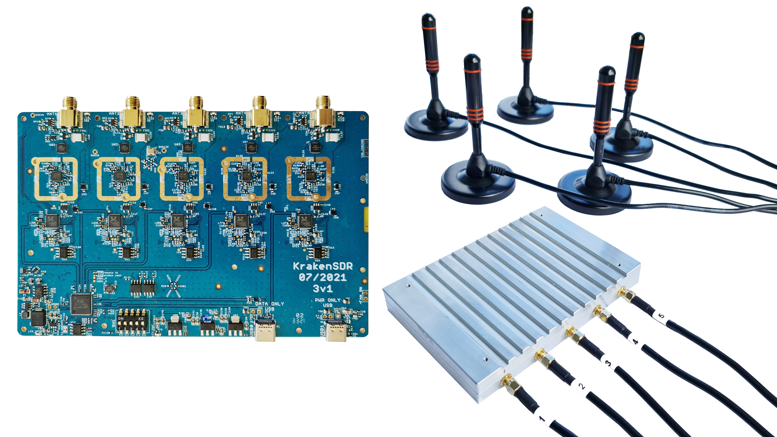
Zoals besproken bestaat een analoge phased array uit een faseverschuiver (en versterker) per kanaal. Dit betekent dat er analoge hardware nodig is naast de SDR. Aan de andere kant kan elke SDR met meer dan één kanaal, waarbij alle kanelen fasegekoppeld zijn en dezelfde klok gebruiken, als een digitale array worden gebruikt. Dit is meestal het geval bij SDR’s met meerdere kanalen. Er zijn veel SDR’s die twee ontvangstkanalen bevatten, zoals de Ettus USRP B210 en de Analog Devices Pluto (het 2e kanaal wordt blootgesteld met een uFL-connector op het bord zelf). Helaas, als je verder gaat dan twee kanalen, kom je in het segment van SDR’s van $10k+ terecht, althans in 2023, zoals de USRP N310. Het grootste probleem is dat goedkope SDR’s meestal niet aan elkaar kunnen worden “gekoppeld” om het aantal kanalen te vermeerderen. De uitzondering is de KerberosSDR (4 kanalen) en KrakenSDR (5 kanalen) die meerdere RTL-SDR’s gebruiken die een LO delen met een gedeelde LO om een goedkope digitale array te vormen; het nadeel is de zeer beperkte bemonsteringsfrequentie (tot 2,56 MHz) en afstemmingsbereik (tot 1766 MHz). De KrakenSDR-kaart en een antenneconfiguratievoorbeeld wordt hieronder getoond.

In dit hoofdstuk zullen we geen specifieke SDR’s gebruiken; in plaats daarvan simuleren we het ontvangen van signalen met Python, en gaan we door de benodigde bewerkingen voor bundelvorming/DOA.

16.3. Introductie Matrix wiskunde in Python/NumPy¶

Python heeft veel voordelen ten opzichte van MATLAB. Het is gratis en open-source en heeft een diversiteit aan toepassingen. Het heeft een levendige gemeenschap, indexen beginnen bij 0 zoals in elke andere taal, het wordt gebruikt binnen AI/ML, en er lijkt een bibliotheek te zijn voor alles wat je maar kunt bedenken. Maar waar Python tekort schiet, is de syntax van matrixmanipulatie (berekenings- /snelheidsgewijs is het snel genoeg, met functies die efficiënt in C/C++ zijn geïmplementeerd). Het helpt ook niet dat er meerdere manieren zijn om matrices in Python te vertegenwoordigen, waarbij de methode np.matrix is verouderd ten gunste van np.ndarray. In dit hoofdstuk geven we een korte inleiding over het uitvoeren van matrixwiskunde in Python met behulp van NumPy, zodat je je comfortabeler voelt wanneer we bij de DOA-voorbeelden komen.

We zullen beginnen met het vervelendste deel van matrixwiskunde met NumPy: vectoren worden behandeld als 1D arrays. Het is dus onmogelijk om onderscheid te maken tussen een rij- of kolomvector (het wordt standaard als een rijvector behandeld). In MATLAB is een vector een 2D-object. In Python kun je een nieuwe vector maken met a = np.array([2,3,4,5]) of een lijst omzetten in een vector met mylist = [2, 3, 4, 5] en dan a = np.asarray(mylist), maar zodra je enige matrixwiskunde wilt doen, is de oriëntatie belangrijk, en a wordt geïnterpreteerd als een rijvector. De vector transponderen met bijv. a.T zal het niet veranderen in een kolomvector! De manier om van een normale vector a een kolomvector te maken, is door a = a.reshape(-1,1) te gebruiken. De -1 vertelt NumPy om de grootte van deze dimensie automatisch te bepalen, terwijl de tweede dimensie lengte 1 behoudt, dus het is vanuit een wiskundig perspectief nog steeds 1D. Het is maar één extra regel, maar het kan de leesbaarheid van matrix code echt verstoren.

Als een kort voorbeeld voor matrixwiskunde in Python zullen we een 3x10 matrix vermenigvuldigen met een 10x1 matrix. Onthoud dat 10x1 10 rijen en 1 kolom betekent. Het is dus een kolomvector omdat het slechts één kolom is. In school hebben we geleerd dat, omdat de binnenste dimensies overeenkomen, dit een geldige matrixvermenigvuldiging is, en dat de resulterende matrix 3x1 groot is (de buitenste dimensies). We zullen np.random.randn() gebruiken om de 3x10 te maken, en np.arange() om de 10x1 te maken:

A = np.random.randn(3,10) # 3x10
B = np.arange(10) # 1D array met lengte 10
B = B.reshape(-1,1) # 10x1
C = A @ B # matrixvermenigvuldiging
print(C.shape) # 3x1
C = C.squeeze() # zie het volgende deel
print(C.shape) # 1D array met lengte 3, makkelijker om te plotten of verder te gebruiken

Na het uitvoeren van matrixwiskunde, kan het resultaat er ongeveer zo uitzien: [[ 0. 0.125 0.251 -0.376 -0.251 ...]]. Deze data heeft duidelijk maar 1 dimensie, maar je kunt het niet doorgeven aan andere functies zoals plot(). Je krijgt een foutmelding of lege grafiek. Dit komt omdat het resultaat technisch gezien een 2D-Pythonarray is. Je moet het naar een 1D-array omzetten met a.squeeze(). De squeeze()-functie verwijdert alle dimensies met lengte 1, en is handig bij het uitvoeren van matrixwiskunde in Python. In het bovenstaande voorbeeld zou het resultaat [ 0. 0.125 0.251 -0.376 -0.251 ...] zijn (let op de ontbrekende tweede haakjes). Dit kan nu verder gebruikt worden om een grafiek te plotten of iets anders te doen.

De beste check die je op je matrixwiskunde kunt uitvoeren is het afdrukken van de dimensies (met A.shape) en te controleren of ze zijn wat je verwacht. Overweeg om de dimensies op elke regel als commentaar te plaatsen, zodat nadien controleren makkelijker wordt.

Hier zijn enkele veelvoorkomende bewerkingen in zowel MATLAB als Python, als een soort spiekbriefje:

Operatie	MATLAB	Python/NumPy
Maak een rijvector met grootte `1 x 4`	`a = [2 3 4 5];`	`a = np.array([2,3,4,5])`
Maak een kolomvector met grootte `4 x 1`	`a = [2; 3; 4; 5];` or `a = [2 3 4 5].'`	`a = np.array([[2],[3],[4],[5]])` or `a = np.array([2,3,4,5])` then `a = a.reshape(-1,1)`
Maak een 2D Matrix	`A = [1 2; 3 4; 5 6];`	`A = np.array([[1,2],[3,4],[5,6]])`
Krijg grootte van een matrix	`size(A)`	`A.shape`
Transponeer matrix $A^T$	`A.'`	`A.T`
Complex Conjugeerde transponatie a.k.a. Conjugeerde Transponatie a.k.a. Hermitische Transponatie a.k.a. $A^H$	`A'`	`A.conj().T` (Helaas is er geen `A.H` voor ndarrays)
Vermenigvulging per element	`A .* B`	`A * B` or `np.multiply(a,b)`
Matrixvermenigvuldiging	`A * B`	`A @ B` or `np.matmul(A,B)`
Inwendig product van twee vectoren (1D)	`dot(a,b)`	`np.dot(a,b)` (gebruik np.dot nooit voor 2D)
Aan elkaar plakken van matrices	`[A A]`	`np.concatenate((A,A))`

16.4. Basiswiskunde¶

Voordat we met de leuke dingen beginnen zullen we eerst een beetje wiskunde moeten behandelen. Het volgende deel is wel zo geschreven dat de wiskunde extreem simpel is met figuren erbij. Alleen de meest basale goniometrische en exponentiële eigenschappen worden gebruikt. Deze basiswiskude is belangrijk om later de pythoncode te begrijpen waarmee we DOA uitvoeren.

We hebben een 1 dimensionale array van antennes die uniform zijn uitgespreid:

Diagram showing direction of arrival (DOA) of a signal impinging on a uniformly spaced antenna array, showing boresight angle and distance between elements or apertures

In dit voorbeeld komt het signaal van rechts dus het raakt het meest rechtste element als eerste. Laten we de vertraging berekenen tussen wanneer het signaal het eerste element raakt en wanneer het het volgende element bereikt. We kunnen dit doen door het volgende trigonometrische probleem te vormen, probeer te begrijpen hoe deze driehoek is gevormd vanuit het bovenstaande figuur. Het rode segment vertegenwoordigt de afstand die het signaal moet afleggen nadat het het eerste element heeft bereikt en voordat het het volgende element raakt.

Trig associated with direction of arrival (DOA) of uniformly spaced array

Als je SOS CAS TOA nog kent, zijn we in dit geval geinteresseerd in de “aanliggende” en hebben we de lengte van de “schuine” ( $d$ ), dus we moeten een cosinus gebruiken:

$\cos(90 - \theta) = \frac{\mathrm{aanliggende}}{\mathrm{schuine}}$

De aanliggende vertelt ons hoe ver het signaal moet reizen tussen het raken van het eerste en het raken van het volgende element, dus het wordt aanliggende $= d \cos(90 - \theta)$ . Nu is er een goniometrische identiteit die ons in staat stelt dit om te zetten in aanliggende $= d \sin(\theta)$ . Dit is slechts een afstand, we moeten dit omzetten in een tijd met behulp van de lichtsnelheid: verstreken tijd $= d \sin(\theta) / c$ [seconden]. Deze vergelijking geldt tussen elk aangrenzend element van onze array, hoewel we het hele ding met een geheel getal kunnen vermenigvuldigen om de niet-aangrenzende elementen te berekenen, omdat ze gelijkmatig verdeeld zijn (dit zullen we later doen).

Nu zullen we deze formules koppelen aan de DSP-wereld. Laten we ons signaal op de basisband $s(t)$ noemen en het verzenden op een bepaalde frequentie, $f_c$ , dus het verzonden signaal is $s(t) e^{2j \pi f_c t}$ . Laten we zeggen dat dit signaal het eerste element op tijd $t = 0$ raakt, wat betekent dat het volgende element na $d \sin(\theta) / c$ [seconden] wordt geraakt, zoals we hierboven hebben berekend. Het tweede element ontvangt dan:

$s(t - \Delta t) e^{2j \pi f_c (t - \Delta t)}$

$\mathrm{waar} \quad \Delta t = d \sin(\theta) / c$

tijdverschuivingen worden afgetrokken van het tijdsargument.

De ontvanger of SDR vermenigvuldigt effectief het signaal met de draaggolf, maar in omgekeerde richting. Na de verschuiving naar de basisband ziet de ontvanger:

$s(t - \Delta t) e^{2j \pi f_c (t - \Delta t)} e^{-2j \pi f_c t}$

$= s(t - \Delta t) e^{-2j \pi f_c \Delta t}$

Met een kleine truc is dit nog verder te vereenvoudigen. Bedenk dat wanneer we een signaal samplen, we dit kunnen modelleren door $t$ te vervangen door $nT$ waar $T$ de sampleperiodetijd is en $n$ gewoon 0, 1, 2, 3… . Door dit in te vullen krijgen we $s(nT - \Delta t) e^{-2j \pi f_c \Delta t}$ . Welnu, $nT$ is zoveel groter dan $\Delta t$ dat we het eerste $\Delta t$ -termijn kunnen weglaten en we $s(nT) e^{-2j \pi f_c \Delta t}$ overhouden. Als de samplefrequentie ooit snel genoeg wordt om de snelheid van het licht over een kleine afstand te benaderen, kunnen we dit opnieuw bekijken, maar onthoud dat onze samplefrequentie slechts een beetje hoger moet zijn dan de bandbreedte van het signaal van belang.

Laten we doorgaan met deze wiskunde maar dingen in discrete termen gaan vertegenwoordigen zodat het meer op onze Python-code lijkt. De laatste vergelijking kan als volgt worden voorgesteld, laten we $\Delta t$ weer invullen:

$s[n] e^{-2j \pi f_c \Delta t}$

$= s[n] e^{-2j \pi f_c d \sin(\theta) / c}$

We zijn bijna klaar. Gelukkig is er nog een vereenvoudiging die we kunnen maken. Herinner je de relatie tussen middenfrequentie en golflengte: $\lambda = \frac{c}{f_c}$ of de vorm die we zullen gebruiken: $f_c = \frac{c}{\lambda}$ . Als we dit invullen krijgen we:

$s[n] e^{-2j \pi \frac{c}{\lambda} d \sin(\theta) / c}$

$= s[n] e^{-2j \pi d \sin(\theta) / \lambda}$

Wat we normaal willen doen met DOA si de afstand tussen twee elementen uit te drukken als een fractie van de golflengte. De meest gekozen waarde tijdens het ontwerpen van een array is om voor $d$ een halve golflengte te gebruiken. Ongeacht wat $d$ is, vanaf dit punt gaan we $d$ uitdrukken als een fractie van de golflengte in plaats van meters, waardoor de vergelijking en al onze code eenvoudiger wordt:

$s[n] e^{-2j \pi d \sin(\theta)}$

Dit is voor aangrenzende elementen, voor het $k$ ’de element moeten we gewoon $d$ keer $k$ vermenigvuldigen:

$s[n] e^{-2j \pi d k \sin(\theta)}$

Nu zijn we klaar! De bovenstaande vergelijking zul je in alle DOA artikelen en implementaties tegenkomen! We noemen die exponentiële term de “array factor” (vaak aangeduid als $a$ ) en stellen het voor als een array, een 1D array voor een 1D antenne array, enz. In Python is $a$ :

a = [np.exp(-2j*np.pi*d*0*np.sin(theta)), np.exp(-2j*np.pi*d*1*np.sin(theta)), np.exp(-2j*np.pi*d*2*np.sin(theta)), ...] # let op de oplopende k
# of
a = np.exp(-2j * np.pi * d * np.arange(Nr) * np.sin(theta)) # Nr is het aantal elementen in de array

Merk op dat het eerste element in een 1+0j resulteert (omdat $e^{0}=1$ ); dit is logisch omdat alles hierboven relatief is aan dat eerste element, dus het ontvangt het signaal zoals het is zonder enige relatieve faseverschuivingen. Dit is puur hoe dat resulteert uit de wiskunde. In werkelijkheid kan elk element als referentie worden beschouwd, maar zoals je later in onze wiskunde/code zult zien, is het verschil in fase/amplitude dat tussen elementen wordt ontvangen wat telt. Het is allemaal relatief.

16.5. Een signaal ontvangen¶

Laten we het bovenstaande concept gebruiken om een ontvangen signaal signaal te simuleren. Voorlopig gebruiken we een enkele toon als verzendsignaal:

import numpy as np
import matplotlib.pyplot as plt

sample_rate = 1e6
N = 10000 # aantal samples om te simuleren

# Maak een toon om het verzonden signaal mee te simuleren
t = np.arange(N)/sample_rate # tijdsvector
f_tone = 0.02e6
tx = np.exp(2j * np.pi * f_tone * t)

Nu gaan we een antenne simuleren, met drie omnidirectionele antennes op een rij, elk een halve golflengte van elkaar verwijderd. We zullen simuleren dat het signaal van de zender op deze array aankomt onder een bepaalde hoek, $\theta$ . Het begrijpen van de factor a, is de reden waarom we al die wiskunde hierboven hebben doorgenomen.

d = 0.5 #afstand van een halve golflengte
Nr = 3
theta_degrees = 20 # aankomstrichting in graden
theta = theta_degrees / 180 * np.pi # naar radialen
a = np.exp(-2j * np.pi * d * np.arange(Nr) * np.sin(theta)) # array factor van hierboven
print(a) # 3 complexe elementen, de eerste is 1+0j

Nu gaan we het signaal ontvangen. Om de array factor toe te passen moeten we een matrixvermenigvuldiging van a en tx uitvoeren, dus laten we beide omzetten naar 2D met de metode die we eerder hebben besproken toen we de matrixwiskunde in Python doornamen. Eerst zetten we het om naar rijvectoren met x.reshape(-1,1). Vervolgens voeren we de matrixvermenigvuldiging uit, aangegeven door het @-symbool. Ook moeten we met een transpositie-operatie tx omzetten van een rijvector naar een kolomvector (zie het als een rotatie van 90 graden), zodat de matrixvermenigvuldiging gelijke binnenste dimensies heeft.

a = a.reshape(-1,1)
print(a.shape) # 3x1
tx = tx.reshape(-1,1)
print(tx.shape) # 10000x1

# matrixvermenigvuldiging
r = a @ tx.T  # laat je niet afleiden door het transponeren, het belangrijkste is dat we de het tx signaal vermenigvuldigen met de a-factor
print(r.shape) # 3x10000.  r  is nu tweedimensionaal: tijd en afstand

Op dit moment is r een 2D array van 3 x 10000 elementen. Dit is omdat we drie array-elementen en 10000 gesimuleerde samples hebben. We kunnen elk individueel signaal eruit halen en de eerste 200 samples laten zien. Hieronder zullen we alleen de reële delen weergeven, maar net als bij elk basisbandsignaal is er ook een imaginair deel. Een vervelend onderdeel van matrixwiskunde in Python is dat we .squeeze() moeten toevoegen oom de extra dimensies met lengte 1 te verwijderen, zodat we naar een normale 1D NumPy-array gaan die we verder kunnen gebruiken.

plt.plot(np.asarray(r[0,:]).squeeze().real[0:200]) # asarray en squeeze zijn helaas noodzakelijk omdat we van een 2D array komen
plt.plot(np.asarray(r[1,:]).squeeze().real[0:200])
plt.plot(np.asarray(r[2,:]).squeeze().real[0:200])
plt.show()

Note the phase shifts between elements like we expect to happen (unless the signal arrives at boresight in which case it will reach all elements at the same time and there wont be a shift, set theta to 0 to see). Element 0 appears to arrive first, with the others slightly delayed. Try adjusting the angle and see what happens.

As one final step, let’s add noise to this received signal, as every signal we will deal with has some amount of noise. We want to apply the noise after the array factor is applied, because each element experiences an independent noise signal (we can do this because AWGN with a phase shift applied is still AWGN):

n = np.random.randn(Nr, N) + 1j*np.random.randn(Nr, N)
r = r + 0.5*n # r and n are both 3x10000

../_images/doa_time_domain_with_noise.svg

16.6. Conventional DOA¶

We will now process these samples r, pretending we don’t know the angle of arrival, and perform DOA, which involves estimating the angle of arrival(s) with DSP and some Python code! As discussed earlier in this chapter, the act of beamforming and performing DOA are very similar and are often built off the same techniques. Throughout the rest of this chapter we will investigate different “beamformers”, and for each one we will start with the beamformer math/code that calculates the weights, $w$ . These weights can be “applied” to the incoming signal r through the simple equation $w^H r$ , or in Python w.conj().T @ r. In the example above, r is a 3x10000 matrix, but after we apply the weights we are left with 1x10000, as if our receiver only had one antenna, and we can use normal RF DSP to process the signal. After developing the beamformer, we will apply that beamformer to the DOA problem.

We’ll start with the “conventional” beamforming approach, a.k.a. delay-and-sum beamforming. Our weights vector w needs to be a 1D array for a uniform linear array, in our example of three elements, w is a 3x1 array of complex weights. With conventional beamforming we leave the magnitude of the weights at 1, and adjust the phases so that the signal constructively adds up in the direction of our desired signal, which we will refer to as $\theta$ . It turns out that this is the exact same math we did above!

$w_{conventional} = e^{-2j \pi d k \sin(\theta)}$

or in Python:

w = np.exp(-2j * np.pi * d * np.arange(Nr) * np.sin(theta)) # Conventional, aka delay-and-sum, beamformer
r = w.conj().T @ r # example of applying the weights to the received signal (i.e., perform the beamforming)

where Nr is the number of elements in our uniform linear array with spacing of d fractions of wavelength (most often ~0.5). As you can see, the weights don’t depend on anything other than the array geometry and the angle of interest. If our array involved calibrating the phase, we would include those calibration values too.

But how do we know the angle of interest theta? We must start by performing DOA, which involves scanning through (sampling) all directions of arrival from -π to +π (-180 to +180 degrees), e.g., in 1 degree increments. At each direction we calculate the weights using a beamformer; we will start by using the conventional beamformer. Applying the weights to our signal r will give us a 1D array of samples, as if we received it with 1 directional antenna. We can then calculate the power in the signal by taking the variance with np.var(), and repeat for every angle in our scan. We will plot the results and look at it with our human eyes/brain, but what most RF DSP does is find the angle of maximum power (with a peak-finding algorithm) and call it the DOA estimate.

theta_scan = np.linspace(-1*np.pi, np.pi, 1000) # 1000 different thetas between -180 and +180 degrees
results = []
for theta_i in theta_scan:
   w = np.exp(-2j * np.pi * d * np.arange(Nr) * np.sin(theta_i)) # Conventional, aka delay-and-sum, beamformer
   r_weighted = w.conj().T @ r # apply our weights. remember r is 3x10000
   results.append(10*np.log10(np.var(r_weighted))) # power in signal, in dB so its easier to see small and large lobes at the same time
results -= np.max(results) # normalize

# print angle that gave us the max value
print(theta_scan[np.argmax(results)] * 180 / np.pi) # 19.99999999999998

plt.plot(theta_scan*180/np.pi, results) # lets plot angle in degrees
plt.xlabel("Theta [Degrees]")
plt.ylabel("DOA Metric")
plt.grid()
plt.show()

../_images/doa_conventional_beamformer.svg

We found our signal! You’re probably starting to realize where the term electrically steered array comes in. Try increasing the amount of noise to push it to its limit, you might need to simulate more samples being received for low SNRs. Also try changing the direction of arrival.

If you prefer viewing angle on a polar plot, use the following code:

fig, ax = plt.subplots(subplot_kw={'projection': 'polar'})
ax.plot(theta_scan, results) # MAKE SURE TO USE RADIAN FOR POLAR
ax.set_theta_zero_location('N') # make 0 degrees point up
ax.set_theta_direction(-1) # increase clockwise
ax.set_rlabel_position(55)  # Move grid labels away from other labels
plt.show()

Example polar plot of performing direction of arrival (DOA) showing the beam pattern and 180 degree ambiguity

We will keep seeing this pattern of looping over angles, and having some method of calculating the beamforming weights, then applying them to the recieved signal. In the next beamforming method (MVDR) we will use our received signal r as part of the weight calculations, making it an adaptive technique. But first we will investigate some interesting things that happen with phased arrays, including why we have that second peak at 160 degrees.

16.7. 180 Degree Ambiguity¶

Let’s talk about why is there a second peak at 160 degrees; the DOA we simulated was 20 degrees, but it is not a coincidence that 180 - 20 = 160. Picture three omnidirectional antennas in a line placed on a table. The array’s boresight is 90 degrees to the axis of the array, as labeled in the first diagram in this chapter. Now imagine the transmitter in front of the antennas, also on the (very large) table, such that its signal arrives at a +20 degree angle from boresight. Well the array sees the same effect whether the signal is arriving with respect to its front or back, the phase delay is the same, as depicted below with the array elements in red and the two possible transmitter DOA’s in green. Therefore, when we perform the DOA algorithm, there will always be a 180 degree ambiguity like this, the only way around it is to have a 2D array, or a second 1D array positioned at any other angle w.r.t the first array. You may be wondering if this means we might as well only calculate -90 to +90 degrees to save compute cycles, and you would be correct!

16.8. Broadside of the Array¶

To demonstrate this next concept, let’s try sweeping the angle of arrival (AoA) from -90 to +90 degrees instead of keeping it constant at 20:

Animation of direction of arrival (DOA) showing the broadside of the array

As we approach the broadside of the array (a.k.a. endfire), which is when the signal arrives at or near the axis of the array, performance drops. We see two main degradations: 1) the main lobe gets wider and 2) we get ambiguity and don’t know whether the signal is coming from the left or the right. This ambiguity adds to the 180 degree ambiguity discussed earlier, where we get an extra lobe at 180 - theta, causing certain AoA to lead to three lobes of roughly equal size. This broadside ambiguity makes sense though, the phase shifts that occur between elements are identical whether the signal arrives from the left or right side w.r.t. the array axis. Just like with the 180 degree ambiguity, the solution is to use a 2D array or two 1D arrays at different angles. In general, beamforming works best when the angle is closer to the boresight.

16.9. When d is not λ/2¶

So far we have been using a distance between elements, d, equal to one half wavelength. So for example, an array designed for 2.4 GHz WiFi with λ/2 spacing would have a spacing of 3e8/2.4e9/2 = 12.5cm or about 5 inches, meaning a 4x4 element array would be about 15” x 15” x the height of the antennas. There are times when an array may not be able to achieve exactly λ/2 spacing, such as when space is restricted, or when the same array has to work on a variety of carrier frequencies.

Let’s examine when the spacing is greater than λ/2, i.e., too much spacing, by varying d between λ/2 and 4λ. We will remove the bottom half of the polar plot since it’s a mirror of the top anyway.

Animation of direction of arrival (DOA) showing what happens when distance d is much more than half-wavelength

As you can see, in addition to the 180 degree ambiguity we discussed earlier, we now have additional ambiguity, and it gets worse as d gets higher (extra/incorrect lobes form). These extra lobes are known as grating lobes, and they are a result of “spatial aliasing”. As we learned in the IQ-sampling chapter, when we don’t sample fast enough we get aliasing. The same thing happens in the spatial domain; if our elements are not spaced close enough together w.r.t. the carrier frequency of the signal being observed, we get garbage results in our analysis. You can think of spacing out antennas as sampling space! In this example we can see that the grating lobes don’t get too problematic until d > λ, but they will occur as soon as you go above λ/2 spacing.

Now what happens when d is less than λ/2, such as when we need to fit the array in a small space? Let’s repeat the same simulation:

Animation of direction of arrival (DOA) showing what happens when distance d is much less than half-wavelength

While the main lobe gets wider as d gets lower, it still has a maximum at 20 degrees, and there are no grating lobes, so in theory this would still work (at least at high SNR). To better understand what breaks as d gets too small, let’s repeat the experiment but with an additional signal arriving from -40 degrees:

Animation of direction of arrival (DOA) showing what happens when distance d is much less than half-wavelength and there are two signals present

Once we get lower than λ/4 there is no distinguishing between the two different paths, and the array performs poorly. As we will see later in this chapter, there are beamforming techniques that provide more precise beams than conventional beamforming, but keeping d as close to λ/2 as possible will continue to be a theme.

16.10. MVDR/Capon Beamformer¶

We will now look at a beamformer that is slightly more complicated than the conventional/delay-and-sum technique, but tends to perform much better, called the Minimum Variance Distortionless Response (MVDR) or Capon Beamformer. Recall that variance of a signal corresponds to how much power is in the signal. The idea behind MVDR is to keep the signal at the angle of interest at a fixed gain of 1 (0 dB), while minimizing the total variance/power of the resulting beamformed signal. If our signal of interest is kept fixed then minimizing the total power means minimizing interferers and noise as much as possible. It is often refered to as a “statistically optimal” beamformer.

The MVDR/Capon beamformer can be summarized in the following equation:

$w_{mvdr} = \frac{R^{-1} a}{a^H R^{-1} a}$

where $R$ is the covariance matrix estimate based on our recieved samples, calculated by multiplying r with the complex conjugate transpose of itself, i.e., $R = r r^H$ , and the result will be a Nr x Nr size matrix (3x3 in the examples we have seen so far). This covariance matrix tells us how similar the samples received from the three elements are. The vector $a$ is the steering vector corresponding to the desired direction and was discussed at the beginning of this chapter.

If we already know the direction of the signal of interest, and that direction does not change, we only have to calculate the weights once and simply use them to receive our signal of interest. Although even if the direction doesn’t change, we benefit from recalculating these weights periodically, to account for changes in the interference/noise, which is why we refer to these non-conventional digital beamformers as “adaptive” beamforming; they use information in the signal we receive to calculate the best weights. Just as a reminder, we can perform beamforming using MVDR by calculating these weights and applying them to the signal with w.conj().T @ r, just like we did in the conventional method, the only difference is how the weights are calculated.

To perform DOA using the MVDR beamformer, we simply repeat the MVDR calculation while scanning through all angles of interest. I.e., we act like our signal is coming from angle $\theta$ , even if it isn’t. At each angle we calculate the MVDR weights, then apply them to the received signal, then calculate the power in the signal. The angle that gives us the highest power is our DOA estimate, or even better we can plot power as a function of angle to see the beam pattern, as we did above with the conventional beamformer, that way we don’t need to assume how many signals are present.

In Python we can implement the MVDR/Capon beamformer as follows, which will be done as a function so that it’s easy to use later on:

# theta is the direction of interest, in radians, and r is our received signal
def w_mvdr(theta, r):
   a = np.exp(-2j * np.pi * d * np.arange(Nr) * np.sin(theta)) # steering vector in the desired direction theta
   a = a.reshape(-1,1) # make into a column vector (size 3x1)
   R = r @ r.conj().T # Calc covariance matrix. gives a Nr x Nr covariance matrix of the samples
   Rinv = np.linalg.pinv(R) # 3x3. pseudo-inverse tends to work better/faster than a true inverse
   w = (Rinv @ a)/(a.conj().T @ Rinv @ a) # MVDR/Capon equation! numerator is 3x3 * 3x1, denominator is 1x3 * 3x3 * 3x1, resulting in a 3x1 weights vector
   return w

Using this MVDR beamformer in the context of DOA, we get the following Python example:

theta_scan = np.linspace(-1*np.pi, np.pi, 1000) # 1000 different thetas between -180 and +180 degrees
results = []
for theta_i in theta_scan:
   w = w_mvdr(theta_i, r) # 3x1
   r_weighted = w.conj().T @ r # apply weights
   power_dB = 10*np.log10(np.var(r_weighted)) # power in signal, in dB so its easier to see small and large lobes at the same time
   results.append(power_dB)
results -= np.max(results) # normalize

When applied to the previous DOA example simulation, we get the following:

It appears to work fine, but to really compare this to other techniques we’ll have to create a more interesting problem. Let’s set up a simulation with an 8-element array receiving three signals from different angles: 20, 25, and 40 degrees, with the 40 degree one received at a much lower power than the other two, as a way to spice things up. Our goal will be to detect all three signals, meaning we want to be able to see noticeable peaks (high enough for a peak-finder algorithm to extract). The code to generate this new scenario is as follows:

Nr = 8 # 8 elements
theta1 = 20 / 180 * np.pi # convert to radians
theta2 = 25 / 180 * np.pi
theta3 = -40 / 180 * np.pi
a1 = np.exp(-2j * np.pi * d * np.arange(Nr) * np.sin(theta1)).reshape(-1,1) # 8x1
a2 = np.exp(-2j * np.pi * d * np.arange(Nr) * np.sin(theta2)).reshape(-1,1)
a3 = np.exp(-2j * np.pi * d * np.arange(Nr) * np.sin(theta3)).reshape(-1,1)
# we'll use 3 different frequencies.  1xN
tone1 = np.exp(2j*np.pi*0.01e6*t).reshape(1,-1)
tone2 = np.exp(2j*np.pi*0.02e6*t).reshape(1,-1)
tone3 = np.exp(2j*np.pi*0.03e6*t).reshape(1,-1)
r = a1 @ tone1 + a2 @ tone2 + 0.1 * a3 @ tone3
n = np.random.randn(Nr, N) + 1j*np.random.randn(Nr, N)
r = r + 0.05*n # 8xN

You can put this code at the top of your script, since we are generating a different signal than the original example. If we run our MVDR beamformer on this new scenario we get the following results:

It works pretty well, we can see the two signals received only 5 degrees apart, and we can also see the 3rd signal (at -40 or 320 degrees) that was received at one tenth the power of the others. Now let’s run the conventional beamformer on this new scenario:

While it might be a pretty shape, it’s not finding all three signals at all… By comparing these two results we can see the benefit from using a more complex and “adptive” beamformer.

As a quick aside for the interested reader, there is actually an optimization that can be made when performing DOA with MVDR, using a trick. Recall that we calculate the power in a signal by taking the variance, which is the mean of the magnitude squared (assuming our signals average value is zero which is almost always the case for baseband RF). We can represent taking the power in our signal after applying our weights as:

$P_{mvdr} = \frac{1}{N} \sum_{n=0}^{N-1} \left| w^H_{mvdr} r_n \right|^2$

If we plug in the equation for the MVDR weights we get:

$P_{mvdr} = \frac{1}{N} \sum_{n=0}^{N-1} \left| \left( \frac{R^{-1} a}{a^H R^{-1} a} \right)^H r_n \right|^2 = \frac{1}{N} \sum_{n=0}^{N-1} \left| \frac{a^H R^{-1}}{a^H R^{-1} a} r_n \right|^2 ... \mathrm{math} = \frac{1}{a^H R^{-1} a}$

Meaning we don’t have to apply the weights at all, this final equation above for power can be used directly in our DOA scan, saving us some computations:

def power_mvdr(theta, r):
    a = np.exp(-2j * np.pi * d * np.arange(r.shape[0]) * np.sin(theta)) # steering vector in the desired direction theta_i
    a = a.reshape(-1,1) # make into a column vector (size 3x1)
    R = r @ r.conj().T # Calc covariance matrix. gives a Nr x Nr covariance matrix of the samples
    Rinv = np.linalg.pinv(R) # 3x3. pseudo-inverse tends to work better than a true inverse
    return 1/(a.conj().T @ Rinv @ a).squeeze()

To use this in the previous simulation, within the for loop, the only thing left to do is take the 10*np.log10() and you’re done, there are no weights to apply; we skipped calculating the weights!

There are many more beamformers out there, but next we are going to take a moment to discuss how the number of elements impacts our ability to perform beamforming and DOA.

16.11. Number of Elements¶

Coming soon!

16.12. MUSIC¶

We will now change gears and talk about a different kind of beamformer. All of the previous ones have fallen in the “delay-and-sum” category, but now we will dive into “sub-space” methods. These involve dividing the signal subspace and noise subspace, which means we must estimate how many signals are being received by the array, to get a good result. MUltiple SIgnal Classification (MUSIC) is a very popular sub-space method that involves calculating the eigenvectors of the covariance matrix (which is a computationally intensive operation by the way). We split the eigenvectors into two groups: signal sub-space and noise-subspace, then project steering vectors into the noise sub-space and steer for nulls. That might seem confusing at first, which is part of why MUSIC seems like black magic!

The core MUSIC equation is the following:

$\hat{\theta} = \mathrm{argmax}\left(\frac{1}{a^H V_n V^H_n a}\right)$

where $V_n$ is that list of noise sub-space eigenvectors we mentioned (a 2D matrix). It is found by first calculating the eigenvectors of $R$ , which is done simply by w, v = np.linalg.eig(R) in Python, and then splitting up the vectors (w) based on how many signals we think the array is receiving. There is a trick for estimating the number of signals that we’ll talk about later, but it must be between 1 and Nr - 1. I.e., if you are designing an array, when you are choosing the number of elements you must have one more than the number of anticipated signals. One thing to note about the equation above is $V_n$ does not depend on the array factor $a$ , so we can precalculate it before we start looping through theta. The full MUSIC code is as follows:

num_expected_signals = 3 # Try changing this!

# part that doesn't change with theta_i
R = r @ r.conj().T # Calc covariance matrix, it's Nr x Nr
w, v = np.linalg.eig(R) # eigenvalue decomposition, v[:,i] is the eigenvector corresponding to the eigenvalue w[i]
eig_val_order = np.argsort(np.abs(w)) # find order of magnitude of eigenvalues
v = v[:, eig_val_order] # sort eigenvectors using this order
# We make a new eigenvector matrix representing the "noise subspace", it's just the rest of the eigenvalues
V = np.zeros((Nr, Nr - num_expected_signals), dtype=np.complex64)
for i in range(Nr - num_expected_signals):
   V[:, i] = v[:, i]

theta_scan = np.linspace(-1*np.pi, np.pi, 1000) # -180 to +180 degrees
results = []
for theta_i in theta_scan:
    a = np.exp(-2j * np.pi * d * np.arange(Nr) * np.sin(theta_i)) # array factor
    a = a.reshape(-1,1)
    metric = 1 / (a.conj().T @ V @ V.conj().T @ a) # The main MUSIC equation
    metric = np.abs(metric.squeeze()) # take magnitude
    metric = 10*np.log10(metric) # convert to dB
    results.append(metric)

results /= np.max(results) # normalize

Running this algorithm on the complex scenario we have been using, we get the following very precise results, showing the power of MUSIC:

Example of direction of arrival (DOA) using MUSIC algorithm beamforming

Now what if we had no idea how many signals were present? Well there is a trick; you sort the eigenvalue magnitudes from highest to lowest, and plot them (it may help to plot them in dB):

plot(10*np.log10(np.abs(w)),'.-')

The eigenvalues associated with the noise-subspace are going to be the smallest, and they will all tend around the same value, so we can treat these low values like a “noise floor”, and any eigenvalue above the noise floor represents a signal. Here we can clearly see there are three signals being received, and adjust our MUSIC algorithm accordingly. If you don’t have a lot of IQ samples to process or the signals are at low SNR, the number of signals might not be as obvious. Feel free to play around by adjusting num_expected_signals between 1 and 7, you’ll find that underestimating the number will lead to missing signal(s) while overestimating will only slightly hurt performance.

Another experiment worth trying with MUSIC is to see how close two signals can arrive at (in angle) while still distinguishing between them; sub-space techniques are especially good at that. The animation below shows an example, with one signal at 18 degrees and another slowly sweeping angle of arrival.

16.13. ESPRIT¶

Coming soon!

16.14. Radar-Style Scenario¶

In all of the previous DOA examples, we had one or more signals and we were interested in finding the directions of all of them. Now we will shift gears to a more radar-oriented scenario, where you have an environment with noise and interferers, and then a signal of interest (SOI) that is only present during certain times. A training phase, occurring when you know the SOI is not present, is performed, to capture the characteristics of the interference. We will be using the MVDR beamformer.

A new scenario is used in the Python simulation below, involving one jammer and one SOI. In addition to simulating the samples of both signals combined (with noise), we also simulate just the jammer (with noise), which represents samples taken before the SOI was present. The received samples r that only contain the jammer, are used as part of a training step, where we calculate the R_inv in the MVDR equation. We then “turn on” the SOI by using r that contains both the jammer and SOI, and the rest of the code is the same as normal MVDR DOA, except for one little but important detail- the R_inv’s we use in the MVDR equation have to be:

$w_{mvdr} = \frac{R_{jammer}^{-1} a}{a^H R_{both}^{-1} a}$

The full Python code example is as follows, try tweaking Nr and theta1:

# 1 jammer 1 SOI, generating two different received signals so we can isolate jammer for the training step
Nr = 4 # number of elements
theta1 = 20 / 180 * np.pi # Jammer
theta2 = 30 / 180 * np.pi # SOI
a1 = np.exp(-2j * np.pi * d * np.arange(Nr) * np.sin(theta1)).reshape(-1,1) # Nr x 1
a2 = np.exp(-2j * np.pi * d * np.arange(Nr) * np.sin(theta2)).reshape(-1,1)
tone1 = np.exp(2j*np.pi*0.01*np.arange(N)).reshape(1,-1) # assume sample rate = 1 Hz, its arbitrary
tone2 = np.exp(2j*np.pi*0.02*np.arange(N)).reshape(1,-1)
r_jammer = a1 @ tone1 + 0.1*(np.random.randn(Nr, N) + 1j*np.random.randn(Nr, N))
r_both = a1 @ tone1 + a2 @ tone2 + 0.1*(np.random.randn(Nr, N) + 1j*np.random.randn(Nr, N))

# "Training" step, with just jammer present
Rinv_jammer = np.linalg.pinv(r_jammer @ r_jammer.conj().T) # Nr x Nr, inverse covariance matrix estimate using the received samples

# Now add in the SOI and perform DOA
theta_scan = np.linspace(-1*np.pi, np.pi, 1000) # sweep theta between -180 and +180 degrees
results = []
for theta_i in theta_scan:
    s = np.exp(-2j * np.pi * d * np.arange(Nr) * np.sin(theta_i)) # steering vector in the desired direction theta
    s = s.reshape(-1,1) # make into a column vector (size Nr x 1)
    Rinv_both = np.linalg.pinv(r_both @ r_both.conj().T) # could be outside for loop but more clear having it here
    w = (Rinv_jammer @ s)/(s.conj().T @ Rinv_both @ s) # MVDR/Capon equation!  Note which R's are being used where
    r_weighted = w.conj().T @ r_both # apply weights to the signal that contains both jammer and SOI
    power_dB = 10*np.log10(np.var(r_weighted)) # power in signal, in dB so its easier to see small and large lobes at the same time
    results.append(power_dB)

results -= np.max(results) # normalize

fig, ax = plt.subplots(subplot_kw={'projection': 'polar'})
ax.plot(theta_scan, results)
ax.set_theta_zero_location('N') # make 0 degrees point up
ax.set_theta_direction(-1) # increase clockwise
ax.set_rlabel_position(55)  # Move grid labels away from other labels
ax.set_ylim([-40, 0]) # only plot down to -40 dB

plt.show()

As you can see, there is a peak at the SOI (30 degrees) and null in the direction of the jammer (20 degrees). The jammers null is not as low as the -90 to 0 degree region (which are so low they are not even displayed on the plot), but that’s only because there are no signals coming from that direction, and even though we are nulling the jammer, it’s not perfectly nulled out because it’s so close to the angle of arrival of the SOI and we only simulated 4 elements.

Note that you don’t have to perform full DOA, your goal may be simply to receive the SOI (at an angle you already know) with the interferers nulled out as well as possible, e.g., if you were receiving a radar pulse from a certain direction and wanted to check if it contained energy above a threshold.

16.15. Quiescent Antenna Pattern¶

Recall that our steering vector we keep seeing,

np.exp(-2j * np.pi * d * np.arange(Nr) * np.sin(theta))

encapsulates the array geometry, and its only other parameter is the direction you want to steer towards. We can calculate and plot the “quiescent” antenna pattern (array response) when steered towards a certain direction, which will tell us the arrays natural response if we don’t do any additional beamforming. This can be done by taking the FFT of the complex conjugated weights, no for loop needed. The tricky part is mapping the bins of the FFT output to angle in radians or degrees, which involves an arcsine as you can see in the full example below:

N_fft = 512
theta = theta_degrees / 180 * np.pi # doesnt need to match SOI, we arent processing samples, this is just the direction we want to point at
w = np.exp(-2j * np.pi * d * np.arange(Nr) * np.sin(theta)) # steering vector
w = np.conj(w) # or else our answer will be negative/inverted
w_padded = np.concatenate((w, np.zeros(N_fft - Nr))) # zero pad to N_fft elements to get more resolution in the FFT
w_fft_dB = 10*np.log10(np.abs(np.fft.fftshift(np.fft.fft(w_padded)))**2) # magnitude of fft in dB
w_fft_dB -= np.max(w_fft_dB) # normalize to 0 dB at peak

# Map the FFT bins to angles in radians
theta_bins = np.arcsin(np.linspace(-1, 1, N_fft)) # in radians

# find max so we can add it to plot
theta_max = theta_bins[np.argmax(w_fft_dB)]

fig, ax = plt.subplots(subplot_kw={'projection': 'polar'})
ax.plot(theta_bins, w_fft_dB) # MAKE SURE TO USE RADIAN FOR POLAR
ax.plot([theta_max], [np.max(w_fft_dB)],'ro')
ax.text(theta_max - 0.1, np.max(w_fft_dB) - 4, np.round(theta_max * 180 / np.pi))
ax.set_theta_zero_location('N') # make 0 degrees point up
ax.set_theta_direction(-1) # increase clockwise
ax.set_rlabel_position(55)  # Move grid labels away from other labels
ax.set_thetamin(-90) # only show top half
ax.set_thetamax(90)
ax.set_ylim([-30, 1]) # because there's no noise, only go down 30 dB
plt.show()

It turns out that this pattern is going to almost exactly match the pattern you get when performing DOA with the conventional beamformer (delay-and-sum), when there is a single tone present at theta_degrees and little-to-no noise. The plot may look different because of how low the y-axis gets in dB, or due to the size of the FFT used to create this quiescent response pattern. Try tweaking theta_degrees or the number of elements Nr to see how the response changes.

16.16. 2D DOA¶

Coming soon!

16.17. Steering Nulls¶

Coming soon!

16.18. Conclusion and References¶

All Python code, including code used to generate the figures/animations, can be found on the textbook’s GitHub page.

DOA implementation in GNU Radio - https://github.com/EttusResearch/gr-doa
DOA implementation used by KrakenSDR - https://github.com/krakenrf/krakensdr_doa/blob/main/_signal_processing/krakenSDR_signal_processor.py