 Online Python Console
 One-time Donation


20. 2D Beamforming
This chapter extends the 1D beamforming/DOA chapter to 2D arrays. We will start with a simple rectangular array and develop the steering vector equation and MVDR beamformer, then we will work with some actual data from a 3x5 array. Lastly, we will use the interactive tool to explore the effects of different array geometries and element spacing.
Rectangular Arrays and 2D Beamforming
Rectangular arrays (a.k.a. planar arrays) involve a 2D array of elements. With an extra dimension we get some added complexity, but the same basic principles apply, and the hardest part will be visualizing the results (e.g. no more simple polar plots, now we’ll need 3D surface plots). Even though our array is now 2D, that does not mean we have to start adding a dimension to every data structure we’ve been dealing with. For example, we will keep our weights as a 1D array of complex numbers. However, we will need to represent the positions of our elements in 2D. We will keep using theta to refer to the azimuth angle, but now we will introduce a new angle, phi, which is the elevation angle. There are many spherical coordinate conventions, but we will be using the following:

Which corresponds to:
We will also switch to using a generalized steering vector equation, which is not specific to any array geometry:
where \(\boldsymbol{p}\) is the set of element x/y/z positions in meters (size Nr x 3) and \(u\) is the direction we want to point at as a unit vector in x/y/z (size 3x1). In Python this looks like:
def steering_vector(pos, dir):
    #                           Nrx3  3x1
    return np.exp(2j * np.pi * pos @ dir / wavelength) # outputs Nr x 1 (column vector)
Let’s try using this generalized steering vector equation with a simple ULA with 4 elements, to make the connection back to what we have previously learned. We will now represent d in meters instead of relative to wavelength. We will place the elements along the y-axis:
Nr = 4
fc = 5e9
wavelength = 3e8 / fc
d = 0.5 * wavelength # in meters

# We will store our element positions in a list of (x,y,z)'s, even though it's just a ULA along the y-axis
pos = np.zeros((Nr, 3)) # Element positions, as a list of x,y,z coordinates in meters
for i in range(Nr):
    pos[i,0] = 0     # x position
    pos[i,1] = d * i # y position
    pos[i,2] = 0     # z position
The following graphic shows a top-down view of the ULA, with an example theta of 20 degrees.

The only thing left is to connect our old theta with this new unit vector approach. We can calculate dir based on theta pretty easily, we know that the x and z component of our unit vector will be 0 because we are still in 1D space, and based on our spherical coordinate convention the y component will be np.cos(theta), meaning the full code is dir = np.asmatrix([0, np.cos(theta_i), 0]).T. At this point you should be able to connect our generalized steering vector equation with the ULA steering vector equation we have been using. Give this new code a try, pick a theta between 0 and 360 degrees (remember to convert to radians!), and the steering vector should be a 4x1 array.
Now let’s move on to the 2D case. We will place our array in the X-Z plane, with boresight pointing horizontally towards the positive y-axis (\(\theta = 0\), \(\phi = 0\)). We will use the same element spacing as before, but now we will have 16 elements total:
# Now let's switch to 2D, using a 4x4 array with half wavelength spacing, so 16 elements total
Nr = 16

# Element positions, still as a list of x,y,z coordinates in meters, we'll place the array in the X-Z plane
pos = np.zeros((Nr,3))
for i in range(Nr):
    pos[i,0] = d * (i % 4)  # x position
    pos[i,1] = 0            # y position
    pos[i,2] = d * (i // 4) # z position
The top-down view of our rectangular 4x4 array:

In order to point towards a certain theta and phi, we will need to convert those angles into a unit vector. We can use the same generalized steering vector equation as before, but now we will need to calculate the unit vector based on both theta and phi, using the equations at the beginning of this chapter:
# Let's point towards an arbitrary direction
theta = np.deg2rad(60) # azimith angle
phi = np.deg2rad(30) # elevation angle

# Using our spherical coordinate convention, we can calculate the unit vector:
def get_unit_vector(theta, phi):  # angles are in radians
    return np.asmatrix([np.sin(theta) * np.cos(phi), # x component
                        np.cos(theta) * np.cos(phi), # y component
                        np.sin(phi)]).T              # z component

dir = get_unit_vector(theta, phi)
# dir is a 3x1
# [[0.75     ]
#  [0.4330127]
#  [0.5      ]]
Now let’s use our generalized steering vector function to calculate the steering vector:
s = steering_vector(pos, dir)

# Use the conventional beamformer, which is simply the weights equal to the steering vector, plot the beam pattern
w = s # 16x1 vector of weights
At this point it’s worth pointing out that we didn’t actually change the dimensions of anything, going from 1D to 2D, we just have a non-zero x/y/z components, the steering vector equation is still the same and the weights are still a 1D array. It might be tempting to assemble your weights as a 2D array so that visually it matches the array geometry, but it’s not necessary and best to keep it 1D. For every element, there is a corresponding weight, and the list of weights is in the same order as the list of element positions.
Visualizing the beam pattern associated with these weights is a little more complicated because we need a 3D plot or a 2D heatmap. We will scan theta and phi to get a 2D array of power levels, and then plot that using imshow(). The code below does just that, and the result is shown in the figure below, along with a dot at the angle we entered earlier:
resolution = 100 # number of points in each direction
theta_scan = np.linspace(-np.pi/2, np.pi/2, resolution) # azimuth angles
phi_scan = np.linspace(-np.pi/4, np.pi/4, resolution) # elevation angles
results = np.zeros((resolution, resolution)) # 2D array to store results
for i, theta_i in enumerate(theta_scan):
    for j, phi_i in enumerate(phi_scan):
        a = steering_vector(pos, get_unit_vector(theta_i, phi_i)) # array factor
        results[i, j] = np.abs(w.conj().T @ a)[0,0] # power in signal, looks better as linear
plt.imshow(results.T, extent=(theta_scan[0]*180/np.pi, theta_scan[-1]*180/np.pi, phi_scan[0]*180/np.pi, phi_scan[-1]*180/np.pi), origin='lower', aspect='auto', cmap='viridis')
plt.colorbar(label='Power [linear]')
plt.scatter(theta*180/np.pi, phi*180/np.pi, color='red', s=50) # Add a dot at the correct theta/phi
plt.xlabel('Azimuth angle [degrees]')
plt.ylabel('Elevation angle [degrees]')
plt.show()

Let’s simulate some actual samples now; we’ll add two tone jammers arriving from different directions:
N = 10000 # number of samples to simulate

jammer1_theta = np.deg2rad(-30)
jammer1_phi = np.deg2rad(10)
jammer1_dir = get_unit_vector(jammer1_theta, jammer1_phi)
jammer1_s = steering_vector(pos, jammer1_dir) # Nr x 1
jammer1_tone = np.exp(2j*np.pi*0.1*np.arange(N)).reshape(1,-1) # make a row vector

jammer2_theta = np.deg2rad(10)
jammer2_phi = np.deg2rad(50)
jammer2_dir = get_unit_vector(jammer2_theta, jammer2_phi)
jammer2_s = steering_vector(pos, jammer2_dir)
jammer2_tone = np.exp(2j*np.pi*0.2*np.arange(N)).reshape(1,-1) # make a row vector

noise = np.random.normal(0, 1, (Nr, N)) + 1j * np.random.normal(0, 1, (Nr, N)) # complex Gaussian noise
r = jammer1_s @ jammer1_tone + jammer2_s @ jammer2_tone + noise # produces 16 x 10000 matrix of samples
Just for fun let’s calculate the MVDR beamformer weights towards the theta and phi we were using earlier (a unit vector in that direction is still saved as dir):
s = steering_vector(pos, dir) # 16 x 1
R = np.cov(r) # Covariance matrix, 16 x 16
Rinv = np.linalg.pinv(R)
w = (Rinv @ s)/(s.conj().T @ Rinv @ s) # MVDR/Capon equation
Instead of looking at the beam pattern in the crummy 3D plot, we’ll use an alternative method of checking if these weights make sense; we will evaluate the response of the weights towards different directions and calculate the power in dB. Let’s start with the direction we were pointing:
# Power in the direction we are pointing (theta=60, phi=30, which is still saved as dir):
a = steering_vector(pos, dir) # array factor
resp = w.conj().T @ a # scalar
print("Power in direction we are pointing:", 10*np.log10(np.abs(resp)[0,0]), 'dB')
This outputs 0 dB, which is what we expect because MVDR’s goal is to achieve unit gain in the desired direction. Now let’s check the power in the directions of the two jammers, as well as a random direction and a direction that is one degree off of our desired direction (the same code is used, just update dir). The results are shown in the table below:
| Direction Pointed | Gain |
|---|---|
dir (direction used to find MVDR weights) |
0 dB |
| Jammer 1 | -17.488 dB |
| Jammer 2 | -18.551 dB |
1 degree off from dir in both \(\theta\) and \(\phi\) |
-0.00683 dB |
| A random direction | -10.591 dB |
Your results may vary due to the random noise being used to calculate the received samples, which get used to calculate R. But the main take-away is that the jammers will be in a null and very low power, the 1 degree off from dir will be slightly below 0 dB, but still in the main lobe, and then a random direction is going to be lower than 0 dB but higher than the jammers, and very different every run of the simulation. Note that with MVDR you get a gain of 0 dB for the main lobe, but if you were to use the conventional beamformer, you would get \(10 \log_{10}(Nr)\), so about 12 dB for our 16-element array, showing one of the trade-offs of using MVDR.
The code for this section can be found here.
Processing Signals from an Actual 2D Array
In this section we work with some actual data recorded by Jon Kraft using a 3x5 digital array made out of a QUAD-MxFE platform from Analog Devices which supports up to 16 transmit and receive channels (we only used 15 and only in receive mode). Below are some pictures showing the setup, with transmitters labeled.
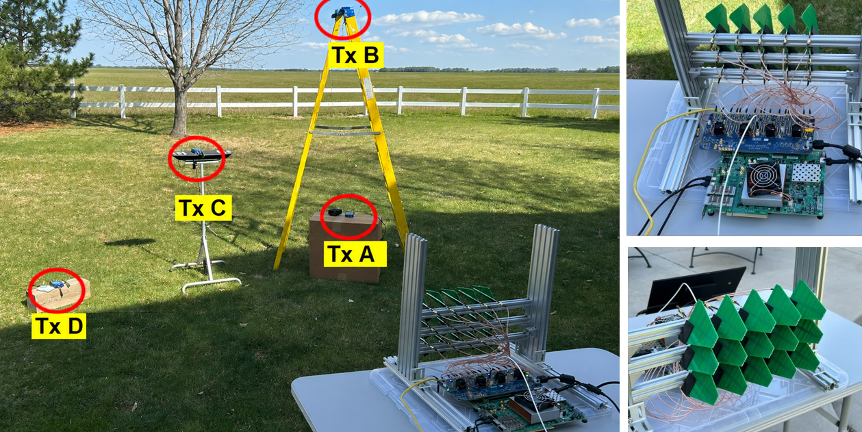
Two downloadable recordings are provided below, the first one contains one emitter located at boresight to the array, which we will use for calibration. The second recording contains two emitters at different directions, which we will use for beamforming and DOA testing.
- IQ recording of just C (used for calibration, as C is at boresight)
- IQ recording of B and D (used for beamforming/DOA testing)
The QUAD-MxFE was tuned to 2.8 GHz and all transmitters were using a simple tone within the observation bandwidth. What’s interesting about this DSP is that it doesn’t actually matter what the sample rate is, none of the array processing techniques we use depend on the sample rate, they just make the assumption that the signal is somewhere in the baseband signal. The DSP does depend on the center frequency, because the phase shift between elements depends on the frequency and angle of arrival. This is opposite of most other signal processing where the sample rate is important, but the center frequency is not.
We can load these recordings into Python using the following code:
import numpy as np
import matplotlib.pyplot as plt

r = np.load("DandB_capture1.npy")[0:15] # 16th element is not connected but was still recorded
r_cal = np.load("C_only_capture1.npy")[0:15] # only the calibration signal (at boresight) on
The spacing between antennas was 0.051 meters. We can represent the element positions as a list of x,y,z coordinates in meters. We will place the array in the X-Z plane, as the array was mounted vertically (with boresight pointing horizontally).
fc = 2.8e9 # center frequency in Hz
d = 0.051 # spacing between antennas in meters
wavelength = 3e8 / fc
Nr = 15
rows = 3
cols = 5

# Element positions, as a list of x,y,z coordinates in meters
pos = np.zeros((Nr, 3))
for i in range(Nr):
        pos[i,0] = d * (i % cols)  # x position
        pos[i,1] = 0 # y position
        pos[i,2] = d * (i // cols) # z position

# Plot and label positions of elements
fig = plt.figure()
ax = fig.add_subplot(projection='3d')
ax.scatter(pos[:,0], pos[:,1], pos[:,2], 'o')
# Label indices
for i in range(Nr):
        ax.text(pos[i,0], pos[i,1], pos[i,2], str(i), fontsize=10)
plt.xlabel("X Position [m]")
plt.ylabel("Y Position [m]")
ax.set_zlabel("Z Position [m]")
plt.grid()
plt.show()
The plot labels each element with its index, which corresponds to the order of the elements in the r and r_cal IQ samples that were recorded.

Calibration is performed using only the r_cal samples, which were recorded with just the transmitter at boresight on. The goal is to find the phase and magnitude offsets for each element. With perfect calibration, and assuming the transmitter was exactly at boresight, all of the individual receive elements should be receiving the same signal, all in phase with each other and at the same magnitude. But because of imperfections in the array/cables/antennas, each element will have a different phase and magnitude offset. The calibration process is to find these offsets, which we will later apply to the r samples before attempting to do any array processing on them.
There are many ways to perform calibration, but we will use a method that involves taking the eigenvalue decomposition of the covariance matrix. The covariance matrix is a square matrix of size Nr x Nr, where Nr is the number of receive elements. The eigenvector corresponding to the largest eigenvalue is the one that represents the received signal, hopefully, and we will use it to find the phase offsets for each element by simply taking the phase of each element of the eigenvector and normalizing it to the first element which we will treat as the reference element. The magnitude calibration does not actually use the eigenvector, but instead uses the mean magnitude of the received signal for each element.
    # Calc covariance matrix, it's Nr x Nr
    R_cal = r_cal @ r_cal.conj().T

# eigenvalue decomposition, v[:,i] is the eigenvector corresponding to the eigenvalue w[i]
    w, v = np.linalg.eig(R_cal)

    # Plot eigenvalues to make sure we have just one large one
    w_dB = 10*np.log10(np.abs(w))
    w_dB -= np.max(w_dB) # normalize
    fig, (ax1) = plt.subplots(1, 1, figsize=(7, 3))
    ax1.plot(w_dB, '.-')
    ax1.set_xlabel('Index')
    ax1.set_ylabel('Eigenvalue [dB]')
    plt.show()

    # Use max eigenvector to calibrate
    v_max = v[:, np.argmax(np.abs(w))]
    mags = np.mean(np.abs(r_cal), axis=1)
    mags = mags[0] / mags # normalize to first element
    phases = np.angle(v_max)
    phases = phases[0] - phases # normalize to first element
    cal_table = mags * np.exp(1j * phases)
    print("cal_table", cal_table)
Below shows the plot of the eigenvalue distribution, we want to make sure that there’s just one large value, and the rest are small, representing one signal being received. Any interferers or multipath will degrade the calibration process.

The calibration table is a list of complex numbers, one for each element, representing the phase and magnitude offsets (it is easier to represent it in rectangular form instead of polar). The first element is the reference element, and will always be 1.0 + 0.j. The rest of the elements are the offsets for each element corresponding to the same order we used for pos.
[1.        +0.j          0.99526771+0.76149029j -0.91754588-0.66825262j
-0.96840297+0.37251012j  0.87866849+0.40446665j  0.56040169+1.50499875j
-0.80109196-1.29299264j -1.28464742-0.31133052j  1.26622038+0.46047599j
 2.01855809+9.77121302j -0.29249322-1.09413205j -1.0372309 -0.17983522j
-0.70614339+0.78682873j -0.75612972+5.67234809j  1.00032754-0.60824109j]
We can apply these offsets to any set of samples recorded from the array simply by multiplying each element of the samples by the corresponding element of the calibration table:
# Apply cal offsets to r
for i in range(Nr):
        r[i, :] *= cal_table[i]
As a side note, this is why we calculated the offsets using mags[0] / mags and phases[0] - phases, if we had reversed that order then we would need to do a division in order to apply the offsets, but we prefer to do the multiplication instead.
Next we will perform DOA estimation using the MUSIC algorithm. We will use the steering_vector() and get_unit_vector() functions we defined earlier to calculate the steering vector for each element of the array, and then use the MUSIC algorithm to estimate the DOA of the two emitters in the r samples. The MUSIC algorithm was discussed in the previous chapter.
# DOA using MUSIC
resolution = 400 # number of points in each direction
theta_scan = np.linspace(-np.pi/2, np.pi/2, resolution) # azimuth angles
phi_scan = np.linspace(-np.pi/4, np.pi/4, resolution) # elevation angles
results = np.zeros((resolution, resolution)) # 2D array to store results
R = np.cov(r) # Covariance matrix, 15 x 15
Rinv = np.linalg.pinv(R)
expected_num_signals = 4
w, v = np.linalg.eig(R) # eigenvalue decomposition, v[:,i] is the eigenvector corresponding to the eigenvalue w[i]
eig_val_order = np.argsort(np.abs(w))
v = v[:, eig_val_order] # sort eigenvectors using this order
V = np.zeros((Nr, Nr - expected_num_signals), dtype=np.complex64) # Noise subspace is the rest of the eigenvalues
for i in range(Nr - expected_num_signals):
        V[:, i] = v[:, i]
for i, theta_i in enumerate(theta_scan):
        for j, phi_i in enumerate(phi_scan):
                dir_i = get_unit_vector(-1*theta_i, phi_i) # TODO figure out why -1* was needed to match reality
                s = steering_vector(pos, dir_i) # 15 x 1
                music_metric = 1 / (s.conj().T @ V @ V.conj().T @ s)
                music_metric = np.abs(music_metric).squeeze()
                music_metric = np.clip(music_metric, 0, 2) # Useful for ABCD one
                results[i, j] = music_metric

results = 10*np.log10(results) # convert to dB

# Keep the top 95%
floor = np.percentile(results, 5)
print("floor:", floor)
results = np.maximum(results, floor)
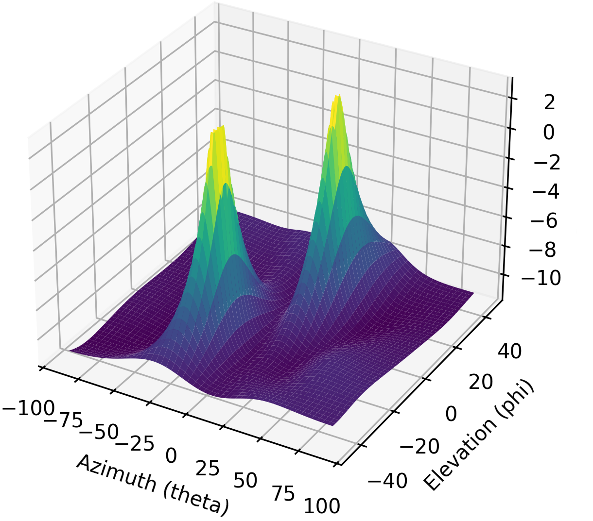
Our results are in 2D, because the array is 2D, so we must either use a 3D plot or a 2D heatmap plot. Let’s try both. First, we will do a 3D plot that has elevation on one axis and azimuth on the other:
# 3D az-el DOA results
fig, ax = plt.subplots(subplot_kw={"projection": "3d", "computed_zorder": False})
surf = ax.plot_surface(np.rad2deg(theta_scan[:,None]), # type: ignore
                                                np.rad2deg(phi_scan[None,:]),
                                                results,
                                                cmap='viridis')
#ax.set_zlim(-10, results[max_idx])
ax.set_xlabel('Azimuth (theta)')
ax.set_ylabel('Elevation (phi)')
ax.set_zlabel('Power [dB]') # type: ignore
fig.savefig('../_images/2d_array_3d_doa_plot.svg', bbox_inches='tight')
plt.show()
Depending on the situation it might be annoying to read off numbers from a 3D plot, so we can also do a 2D heatmap with imshow():
# 2D, az-el heatmap (same as above, but 2D)
extent=(np.min(theta_scan)*180/np.pi,
                np.max(theta_scan)*180/np.pi,
                np.min(phi_scan)*180/np.pi,
                np.max(phi_scan)*180/np.pi)
plt.imshow(results.T, extent=extent, origin='lower', aspect='auto', cmap='viridis') # type: ignore
plt.colorbar(label='Power [linear]')
plt.xlabel('Theta (azimuth, degrees)')
plt.ylabel('Phi (elevation, degrees)')
plt.savefig('../_images/2d_array_2d_doa_plot.svg', bbox_inches='tight')
plt.show()

Using this 2D plot we can easily read off the estimated azimuth and elevation of the two emitters (and see that there was just two). Based on the test setup that was used to produce this recording, these results match reality, the exact azimuth and elevation of the emitters was never actually measured because that would require very specialized equipment.
As an exercise, try using the conventional beamformer, as well as MVDR, and compare the results to MUSIC.
This code in its entirety can be found here.
Interactive Design Tool
The following interactive tool was created by Jason Durbin, a free-lancing phased array engineer, who graciously allowed it to be embedded within PySDR; feel free to visit the full project or his consulting business. This tool allows you to change a phased array’s geometry, element spacing, steering position, add sidelobe tapering, and other features.
Some details on this tool: Antenna elements are assumed to be isotropic. However, the directivity calculation assumes half-hemisphere radiation (e.g. no back lobes). Therefore, the computed directivity will be 3 dBi higher than using pure isotropic (i.e., the individual element gain is +3.0 dBi). The mesh can be made finer by increasing theta/phi, u/v, or azimuth/elevation points. Clicking (or long pressing) elements in the phase/attenuation plots allows you to manually set phase/attenuation (“be sure to select “enable override”). Additionally, the attenuation pop-up allows you to disable elements. Hovering (or touching) the 2D far field plot or geometry plots will show the value of the plot under the cursor.
