13. IQ Files and SigMF

In all our previous Python examples we stored signals as 1D NumPy arrays of type “complex float”. In this chapter we learn how signals can be stored to a file and then read back into Python, as well as introduce the SigMF standard. Storing signal data in a file is extremely useful; you may want to record a signal to a file in order to manually analyze it offline, or share it with a colleague, or build a whole dataset.

Binary Files

Recall that a digital signal at baseband is a sequence of complex numbers.

Example: [0.123 + j0.512, 0.0312 + j0.4123, 0.1423 + j0.06512, …]

These numbers correspond to [I+jQ, I+jQ, I+jQ, I+jQ, I+jQ, I+jQ, I+jQ, …]

When we want to save complex numbers to a file, we save them in the format IQIQIQIQIQIQIQIQ. I.e., we store a bunch of floats in a row, and when we read them back we must separate them back into [I+jQ, I+jQ, …].

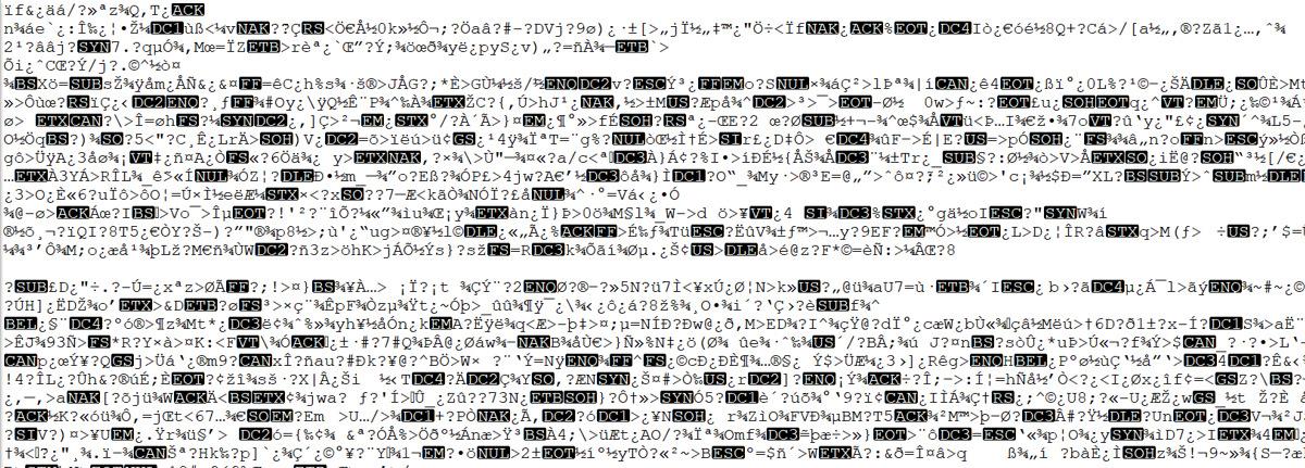
While it’s possible to store the complex numbers in a text file or csv file, we prefer to save them in what’s called a “binary file” to save space. At high sample rates your signal recordings could easily be multiple GB, and we want to be as memory efficient as possible. If you have ever opened a file in a text editor and it looked incomprehensible like the screenshot below, it was probably binary. Binary files contain a series of bytes, and you have to keep track of the format yourself. Binary files are the most efficient way to store data, assuming all possible compression has been performed. Because our signals usually appear like a random sequence of floats, we typically do not attempt to compress the data. Binary files are used for plenty of other things, e.g., compiled programs (called “binaries”). When used to save signals, we call them binary “IQ files”, utilizing the file extension .iq.

In Python, the default complex type is np.complex128, which uses two 64-bit floats per sample. But in DSP/SDR, we tend to use 32-bit floats instead because the ADCs on our SDRs don’t have that much precision to warrant 64-bit floats. In Python we will use np.complex64, which uses two 32-bit floats. When you are simply processing a signal in Python it doesn’t really matter, but when you go to save the 1d array to a file, you want to make sure it’s an array of np.complex64 first.

Python Examples

In Python, and numpy specifically, we use the tofile() function to store a numpy array to a file. Here is a short example of creating a simple QPSK signal plus noise and saving it to a file in the same directory we ran our script from:

import numpy as np
import matplotlib.pyplot as plt

num_symbols = 10000

# x_symbols array will contain complex numbers representing the QPSK symbols. Each symbol will be a complex number with a magnitude of 1 and a phase angle corresponding to one of the four QPSK constellation points (45, 135, 225, or 315 degrees)
x_int = np.random.randint(0, 4, num_symbols) # 0 to 3
x_degrees = x_int*360/4.0 + 45 # 45, 135, 225, 315 degrees
x_radians = x_degrees*np.pi/180.0 # sin() and cos() takes in radians
x_symbols = np.cos(x_radians) + 1j*np.sin(x_radians) # this produces our QPSK complex symbols
n = (np.random.randn(num_symbols) + 1j*np.random.randn(num_symbols))/np.sqrt(2) # AWGN with unity power
r = x_symbols + n * np.sqrt(0.01) # noise power of 0.01
print(r)
plt.plot(np.real(r), np.imag(r), '.')
plt.grid(True)
plt.show()

# Now save to an IQ file
print(type(r[0])) # Check data type.  Oops it's 128 not 64!
r = r.astype(np.complex64) # Convert to 64
print(type(r[0])) # Verify it's 64
r.tofile('qpsk_in_noise.iq') # Save to file

Now examine the details of the file produced and check how many bytes it is. It should be num_symbols * 8 because we used np.complex64, which is 8 bytes per sample, 4 bytes per float (2 floats per sample).

Using a new Python script, we can read in this file using np.fromfile(), like so:

import numpy as np
import matplotlib.pyplot as plt

samples = np.fromfile('qpsk_in_noise.iq', np.complex64) # Read in file.  We have to tell it what format it is
print(samples)

# Plot constellation to make sure it looks right
plt.plot(np.real(samples), np.imag(samples), '.')
plt.grid(True)
plt.show()

A big mistake is to forget to tell np.fromfile() the file format. Binary files don’t include any information about their format. By default, np.fromfile() assumes it is reading in an array of float64s.

Most other languages have methods to read in binary files, e.g., in MATLAB you can use fread(). For visually analyzing an RF file see the section below.

If you ever find yourself dealing with int16’s (a.k.a. short ints), or any other datatype that numpy doesn’t have a complex equivalent for, you will be forced to read the samples in as real, even if they are actually complex. The trick is to read them as real, but then interleave them back into the IQIQIQ… format yourself, a couple different ways of doing this are shown below:

samples = np.fromfile('iq_samples_as_int16.iq', np.int16).astype(np.float32).view(np.complex64)

or

samples = np.fromfile('iq_samples_as_int16.iq', np.int16)
samples /= 32768 # convert to -1 to +1 (optional)
samples = samples[::2] + 1j*samples[1::2] # convert to IQIQIQ...

Coming from MATLAB

If you are trying to switch from MATLAB to Python, you may wonder how to get your MATLAB variables and .mat files saved as binary IQ files. We first need to pick a format type. For example, if our samples are integers between -127 and +127, then we can use 8-bit ints. In this case, we can use the following MATLAB code to save the samples to a binary IQ file:

% let's say our IQ samples are contained in the variable samples
disp(samples(1:20))
filename = 'samples.iq'
fwrite(fopen(filename,'w'), reshape([real(samples);imag(samples)],[],1), 'int8')

You can see all of the allowable format types for fwrite() in the MATLAB documentation. That being said, it is best to stick to 'int8', 'int16', or 'float32'.

On the Python side, you can load in this file using:

samples = np.fromfile('samples.iq', np.int8)
samples = samples[::2] + 1j*samples[1::2]
print(samples[0:20]) # make sure first 20 samples match MATLABs

For 'float32' saved from MATLAB you can use np.complex64 on the Python side, which is interleaved float32’s, and then you can skip the samples[::2] + 1j*samples[1::2] part because numpy will automatically interpret the interleaved floats as complex numbers.

Visually Analyzing an RF File

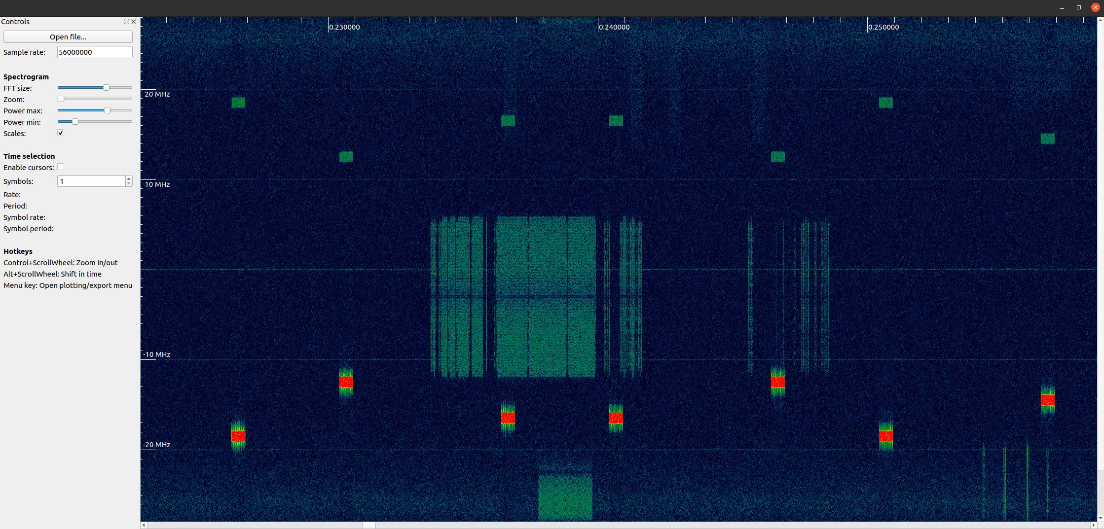
Although we learned how to create our own spectrogram plot in the Frequency Domain Chapter, nothing beats using an already created piece of software. When it comes to analyzing RF recordings without having to install anything, the go-to website is IQEngine which is an entire toolkit for analyzing, processing, and sharing RF recordings.

For those who want a desktop app, there is also inspectrum. Inspectrum is a fairly simple but powerful graphical tool for scanning through an RF file visually, with fine control over the colormap range and FFT size (zoom amount). You can hold alt and use the scroll wheel to shift through time. It has optional cursors to measure the delta-time between two bursts of energy, and the ability to export a slice of the RF file into a new file. For installation on Debian-based platforms such as Ubuntu, use the following commands:

sudo apt-get install qt5-default libfftw3-dev cmake pkg-config libliquid-dev
git clone https://github.com/miek/inspectrum.git
cd inspectrum
mkdir build
cd build
cmake ..
make
sudo make install
inspectrum

Max Values and Saturation

When receiving samples off a SDR it’s important to know the maximum sample value. Many SDRs will output the samples as floats using a maximum value of 1.0 and minimum value of -1.0. Other SDRs will give you samples as integers, usually 16-bit, in which case the max and min values will be +32767 and -32768 (unless otherwise specified), and you can choose to divide by 32,768 to convert them to floats from -1.0 to 1.0. The reason to be aware of the maximum value for your SDR is due to saturation: when receiving an extremely loud signal (or if the gain is set too high), the receiver will “saturate” and it will truncate the high values to whatever the maximum sample value is. The ADCs on our SDRs have a limited number of bits. When making an SDR app it’s wise to always be checking for saturation, and when it happens you should indicate it somehow.

A signal that is saturated will look choppy in the time domain, like this:

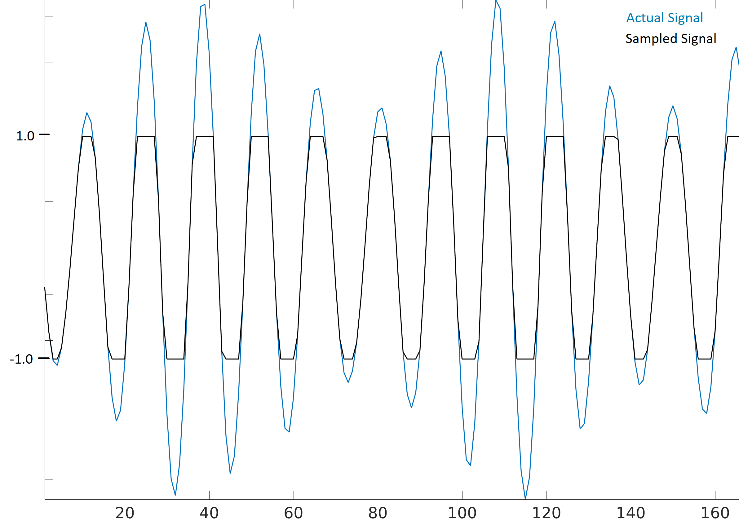
Because of the sudden changes in time domain, due to the truncation, the frequency domain might look smeared. In other words, the frequency domain will include false features; features that resulted from the saturation and are not actually part of the signal, which can throw people off when analyzing a signal.

SigMF and Annotating IQ Files

Since the IQ file itself doesn’t have any metadata associated with it, it’s common to have a 2nd file, containing information about the signal, with the same filename but a .txt or other file extension. This should at a minimum include the sample rate used to collect the signal, and the frequency to which the SDR was tuned. After analyzing the signal, the metadata file could include information about sample ranges of interesting features, such as bursts of energy. The sample index is simply an integer that starts at 0 and increments every complex sample. If you knew that there was energy from sample 492342 to 528492, then you could read in the file and pull out that portion of the array: samples[492342:528493].

Luckily, there is now an open standard that specifies a metadata format used to describe signal recordings, known as SigMF. By using an open standard like SigMF, multiple parties can share RF recordings more easily, and use different tools to operate on the same datasets, such as IQEngine. It also prevents “bitrot” of RF datasets where details of the capture are lost over time due to details of the recording not being collocated with the recording itself.

The most simple (and minimal) way to use the SigMF standard to describe a binary IQ file you have created is to rename the .iq file to .sigmf-data and create a new file with the same name but .sigmf-meta extension, and make sure the datatype field in the meta file matches the binary format of your data file. This meta file is a plaintext file filled with json, so you can simply open it with a text editor and fill it out manually (later we will discuss doing this programmatically). Here is an example .sigmf-meta file you can use as a template:

{
    "global": {
        "core:datatype": "cf32_le",
        "core:sample_rate": 1000000,
        "core:hw": "PlutoSDR with 915 MHz whip antenna",
        "core:author": "Art Vandelay",
        "core:version": "1.0.0"
    },
    "captures": [
        {
            "core:sample_start": 0,
            "core:frequency": 915000000
        }
    ],
    "annotations": []
}

Note the core:cf32_le indicates your .sigmf-data is of type IQIQIQIQ… with 32-bit floats, i.e., np.complex64 like we used previously. Reference the specifications for other available datatypes, such as if you have real data instead of complex, or are using 16-bit integers instead of floats to save space.

Aside from datatype, the most important lines to fill out are core:sample_rate and core:frequency. It is good practice to also enter information about the hardware (core:hw) used to capture the recording, such as the SDR type and antenna, as well as a description of what is known about the signal(s) in the recording in core:description. The core:version is simply the version of the SigMF standard being used at the time the metadata file was created.

If you are capturing your RF recording from within Python, e.g., using the Python API for your SDR, then you can avoid having to manually create these metadata files by using the SigMF Python package. This can be installed on an Ubuntu/Debian based OS as follows:

cd ~
git clone https://github.com/gnuradio/SigMF.git
cd SigMF
sudo pip install .

The Python code to write the .sigmf-meta file for the example towards the beginning of this chapter, where we saved qpsk_in_noise.iq, is shown below:

import numpy as np
import datetime as dt
from sigmf import SigMFFile

# <code from example>

# r.tofile('qpsk_in_noise.iq')
r.tofile('qpsk_in_noise.sigmf-data') # replace line above with this one

# create the metadata
meta = SigMFFile(
    data_file='example.sigmf-data', # extension is optional
    global_info = {
        SigMFFile.DATATYPE_KEY: 'cf32_le',
        SigMFFile.SAMPLE_RATE_KEY: 8000000,
        SigMFFile.AUTHOR_KEY: 'Your name and/or email',
        SigMFFile.DESCRIPTION_KEY: 'Simulation of qpsk with noise',
        SigMFFile.VERSION_KEY: sigmf.__version__,
    }
)

# create a capture key at time index 0
meta.add_capture(0, metadata={
    SigMFFile.FREQUENCY_KEY: 915000000,
    SigMFFile.DATETIME_KEY: dt.datetime.utcnow().isoformat()+'Z',
})

# check for mistakes and write to disk
meta.validate()
meta.tofile('qpsk_in_noise.sigmf-meta') # extension is optional

Simply replace 8000000 and 915000000 with the variables you used to store sample rate and center frequency respectively.

To read in a SigMF recording into Python, use the following code. In this example the two SigMF files should be named qpsk_in_noise.sigmf-meta and qpsk_in_noise.sigmf-data.

from sigmf import SigMFFile, sigmffile

# Load a dataset
filename = 'qpsk_in_noise'
signal = sigmffile.fromfile(filename)
samples = signal.read_samples().view(np.complex64).flatten()
print(samples[0:10]) # lets look at the first 10 samples

# Get some metadata and all annotations
sample_rate = signal.get_global_field(SigMFFile.SAMPLE_RATE_KEY)
sample_count = signal.sample_count
signal_duration = sample_count / sample_rate

For more details reference the SigMF documentation.

A little bonus for those who read this far; the SigMF logo is actually stored as a SigMF recording itself, and when the signal is plotted as a constellation (IQ plot) over time, it produces the following animation:

The Python code used to read in the logo file (located here) and produce the animated GIF above is shown below, for those curious:

import numpy as np
import matplotlib.pyplot as plt
import imageio
from sigmf import SigMFFile, sigmffile

# Load a dataset
filename = 'sigmf_logo' # assume its in the same directory as this script
signal = sigmffile.fromfile(filename)
samples = signal.read_samples().view(np.complex64).flatten()

# Add zeros to the end so its clear when the animation repeats
samples = np.concatenate((samples, np.zeros(50000)))

sample_count = len(samples)
samples_per_frame = 5000
num_frames = int(sample_count/samples_per_frame)
filenames = []
for i in range(num_frames):
    print("frame", i, "out of", num_frames)
    # Plot the frame
    fig, ax = plt.subplots(figsize=(5, 5))
    samples_frame = samples[i*samples_per_frame:(i+1)*samples_per_frame]
    ax.plot(np.real(samples_frame), np.imag(samples_frame), color="cyan", marker=".", linestyle="None", markersize=1)
    ax.axis([-0.35,0.35,-0.35,0.35]) # keep axis constant
    ax.set_facecolor('black') # background color

    # Save the plot to a file
    filename = '/tmp/sigmf_logo_' + str(i) + '.png'
    fig.savefig(filename, bbox_inches='tight')
    filenames.append(filename)

# Create animated gif
images = []
for filename in filenames:
    images.append(imageio.imread(filename))
imageio.mimsave('/tmp/sigmf_logo.gif', images, fps=20)

SigMF Collection for Array Recordings

If you have a phased array, MIMO digital array, TDOA sensors, or any other situation where you are recording multiple channels of synchronized RF data, then you are probably wondering how you store the raw IQ of several streams to file with SigMF. The SigMF Collection system was designed exactly for these applications; a Collection is simply a group of SigMF Recordings (each being one meta and one data file), grouped together using a top-level .sigmf-collection JSON file. This JSON file is fairly straightforward; it needs to have the version of SigMF, an optional description, and then a list of “streams” which is really just the base name of each SigMF Recording in the collection. Here is an example of a .sigmf-collection file:

{
    "collection": {
        "core:version": "1.2.0",
        "core:description": "a 4-element phased array recording",
        "core:streams": [
            {
                "name": "channel-0"
            },
            {
                "name": "channel-1"
            },
            {
                "name": "channel-2"
            },
            {
                "name": "channel-3"
            }
        ]
    }
}

The names of the Recordings don’t have to be channel-0, channel-1, …, they can be whatever you want as long as they are unique and each one corresponds to one data and one meta file. In the above example, this .sigmf-collection file, which we might name 4_element_recording.sigmf-collection for example, needs to be in the same directory as the meta and data files, e.g. in the same directory we would have:

• 4_element_recording.sigmf-collection

• channel-0.sigmf-meta

• channel-0.sigmf-data

• channel-1.sigmf-meta

• channel-1.sigmf-data

• channel-2.sigmf-meta

• channel-2.sigmf-data

• channel-3.sigmf-meta

• channel-3.sigmf-data

You may be thinking this will lead to a huge number of files, for example a 16-element array would lead to 33 files! It is for this reason that SigMF introduced the Archive system, which is really just SigMF’s term for tarballing a set of files. A SigMF Archive file uses the extension .sigmf, not .tar! Many people think that .tar files are compressed, but they are not; they are simply a way to group files together (it’s essentially a file concatenate, no compression involved). You may have seen a .tar.gz file before; this is a tarball that has been compressed with gzip. For our SigMF Archives we won’t bother compressing them, as the data files are already binary and won’t compress much, especially if automatic gain control was used. If you want to create a SigMF Archive in Python, you can tarball all files in a directory together like so:

import tarfile
import os

target_dir = '/mnt/c/Users/marclichtman/Downloads/exampletar/' # SigMF files are here
with tarfile.open(os.path.join(target_dir, '4_element_recording.sigmf'), 'x') as tar: # x means create, but fail if it already exists
    for file in os.listdir(target_dir):
        tar.add(os.path.join(target_dir, file), arcname=file) # arcname makes it not include the full path within the tar

And that’s it! Try (temporarily) renaming .sigmf to .tar and viewing the files in your file browser. To open any of the files in-place (without manually extracting the tar), within Python, you can use:

import tarfile
import json

collection_file = '/mnt/c/Users/marclichtman/Downloads/exampletar/4_element_recording.sigmf'
tar_obj = tarfile.open(collection_file)
print(tar_obj.getnames()) # list of strings of all filenames in the tar
channel_0_meta = tar_obj.extractfile('channel-0.sigmf-meta').read() # read one of the meta files, as an example
channel_0_dict = json.loads(channel_0_meta) # convert to Python dictionary
print(channel_0_dict)

For reading in IQ samples within the tar, instead of np.fromfile(), we’ll use np.frombuffer():

import tarfile
import numpy as np

collection_file = '/mnt/c/Users/marclichtman/Downloads/exampletar/4_element_recording.sigmf'
tar_obj = tarfile.open(collection_file)
channel_0_data_f = tar_obj.extractfile('channel-0.sigmf-data').read() # type bytes
samples = np.frombuffer(channel_0_data_f, dtype=np.int16)
samples = samples[::2] + 1j*samples[1::2] # convert to IQIQIQ...
samples /= 32768 # convert to -1 to +1
print(samples[0:10])

If you want to jump to a different part of the file, you can use tar_obj.extractfile('channel-0.sigmf-data').seek(offset). Then to read a specific number of bytes you use .read(num_bytes). Make sure the number of bytes is a multiple of your datatype!

To sum it up, the following steps should be performed when creating a new SigMF Collection Archive:

1. Create the .sigmf-meta and .sigmf-data file for each channel

2. Create the .sigmf-collection file

3. Tarball all files together into a .sigmf file

4. (Optionally) Share the .sigmf file with others!

Then to read in the recording, just remember you don’t have to extract the tarball, you can read the files in-place.