19. Beamforming & DOA¶

In this chapter we cover the concepts of beamforming, direction-of-arrival (DOA), and phased arrays in general. We compare the different types and geometries of arrays, and how element spacing plays a vital role. Techniques such as MVDR/Capon and MUSIC are introduced and demonstrated using Python simulation examples.

Beamforming Overview¶

A phased array, a.k.a. electronically steered array, is an array/collection of antennas that can be used on the transmit or receive side in both communications and radar systems. You’ll find phased arrays on ground-based systems, airborne, and on satellites. We typically refer to the antennas that make up an array as elements, and sometimes the array is called a “sensor” instead. These array elements are most often omnidirectional antennas, equally spaced in either a line or across two dimensions.

Beamforming is a signal processing operation used with antenna arrays to create a spatial filter; it filters out signals from all directions except the desired direction(s). Beamforming can be used to increase SNR of desired signals, null out interferers, shape beam patterns, or even transmit/receive multiple data streams at the same time and frequency. As part of beamforming we use weights (a.k.a. coefficients) applied to each element of an array, either digitally or in analog circuitry. We manipulate the weights to form the beam(s) of the array, hence the name beamforming! We can steer these beams (and nulls) extremely fast; much faster than mechanically gimballed antennas, which can be thought of as an alternative to phased arrays. We’ll typically discuss beamforming within the context of a communications link, where the receiver aims to receive one or more signals at the greatest possible SNR. Arrays also have a huge role in radar, where the goal is to detect and track targets.

Diagram showing a complex scenario of multiple signals arriving at an array

Beamforming approaches can be broken down into three categories, namely: conventional, adaptive, and blind. Conventional beamforming is most useful when you already know the direction of arrival of the signal of interest, and the beamforming process involves choosing weights to maximize the array gain in that direction. This can be used on both the receive or transmit side of a communication system. Adaptive beamforming, on the other hand, typically involves adjusting the weights based on the beamformer’s input, to optimize some criteria (e.g., nulling out an interferer, having multiple main beams, etc.). Due to the closed loop and adaptive nature, adaptive beamforming is typically just used on the receive side, so the “beamformer’s input” is simply your received signal, and adaptive beamforming involves adjusting the weights based on the statistics of that received data.

The following taxonomy attempts to categorize the many areas of beamforming while providing example techniques:

A beamforming taxonomy, categorizing beamforming into conventional, adaptive, and blind, as well as showing how direction of arrival (DOA) estimation fits in

Direction-of-Arrival Overview¶

Direction-of-Arrival (DOA) within DSP/SDR refers to the process of using an array of antennas to detect and estimate the directions of arrival of one or more signals received by that array (versus beamforming, which is focused on the process of receiving a signal while rejecting as much noise and interference). Although DOA certainly falls under the beamforming topic umbrella, the two terms can get confusing. Some techniques such as Conventional and MVDR beamforming can apply to both DOA and beamforming, because the same technique used for beamforming is used to perform DOA by sweeping the angle of interest and performing the beamforming operation at each angle, then looking for peaks in the result (each peak is a signal, but we don’t know whether it is the signal of interest, an interferer, or even a multipath bounce from the signal of interest). You can think of these DOA techniques as a wrapper around a specific beamformer. Other beamformers are unable to be simply wrapped into a DOA routine, such as due to extra inputs that won’t be available within the context of DOA. There are also DOA techniques such as MUSIC and ESPIRT which are strictly for the purpose of DOA and are not beamformers. Because most beamforming techniques assume you know the angle of arrival of the signal of interest, if the target is moving, or the array is moving, you will have to continuously perform DOA as an intermediate step, even if your primary goal is to receive and demodulate the signal of interest.

Phased arrays and beamforming/DOA find use in all sorts of applications, although you will most often see them used in multiple forms of radar, newer WiFi standards, mmWave communication within 5G, satellite communications, and jamming. Generally, any applications that require a high-gain antenna, or require a rapidly moving high-gain antenna, are good candidates for phased arrays.

Types of Arrays¶

Phased arrays can be broken down into three types:

Analog, a.k.a. passive electronically scanned array (PESA) or traditional phased arrays, where analog phase shifters are used to steer the beam. On the receive side, all elements are summed after phase shifting (and optionally, adjustable gain) and turned into a signal channel which is downconverted and received. On the transmit side the inverse takes place; a single digital signal is outputted from the digital side, and on the analog side phase shifters and gain stages are used to produce the output going to each antenna. These digital phase shifters will have a limited number of bits of resolution, and control latency.
Digital, a.k.a. active electronically scanned array (AESA), where every single element has its own RF front end, and the beamforming is done entirely in the digital domain. This is the most expensive approach, as RF components are expensive, but it provides much more flexibility and speed than PESAs. Digital arrays are popular with SDRs, although the number of receive or transmit channels of the SDR limits the number of elements in your array.
Hybrid, where the array consists of many subarrays that individually resemble analog arrays, where each subarray has its own RF front-end just like with digital arrays. This is the most common approach for modern phased arrays, as it provides the best of both worlds.

Note that the terms PESA and AESA are mainly just used in the context of radar, and there is some ambiguity when it comes to exactly what constitutes a PESA or AESA. Therefore, using the terms analog/digital/hybrid array is clearer and can be applied to any type of application.

A real-world example of each type is shown below:

Example of phased arrays including Passive electronically scanned array (PESA), Active electronically scanned array (AESA), Hybrid array, showing Raytheon's MIM-104 Patriot Radar, ELM-2084 Israeli Multi-Mission Radar, Starlink User Terminal, aka Dishy

In addition to these three types, there is also the geometry of the array. The simplest geometry is the uniform linear array (ULA) where the antennas are in a straight line with equal spacing (i.e., in 1 dimension). ULAs suffer from a 180-degree ambiguity, which we will talk about later, and one solution is to place the antennas in a circle, which we call a uniform circular array (UCA). Lastly, for 2D beams, we usually use a uniform rectangular array (URA), where the antennas are in a grid pattern.

In this chapter we focus on digital arrays, as they are more suited towards simulation and DSP, but the concepts carry over to analog and hybrid. In the next chapter we get hands-on with the “Phaser” SDR from Analog Devices that has a 10 GHz 8-element analog array with phase and gain shifters, connected to a Pluto and Raspberry Pi. We will also focus on the ULA geometry because it provides the simplest math and code, but all of the concepts carry over to other geometries, and at the end of the chapter we touch upon the UCA.

SDR Requirements¶

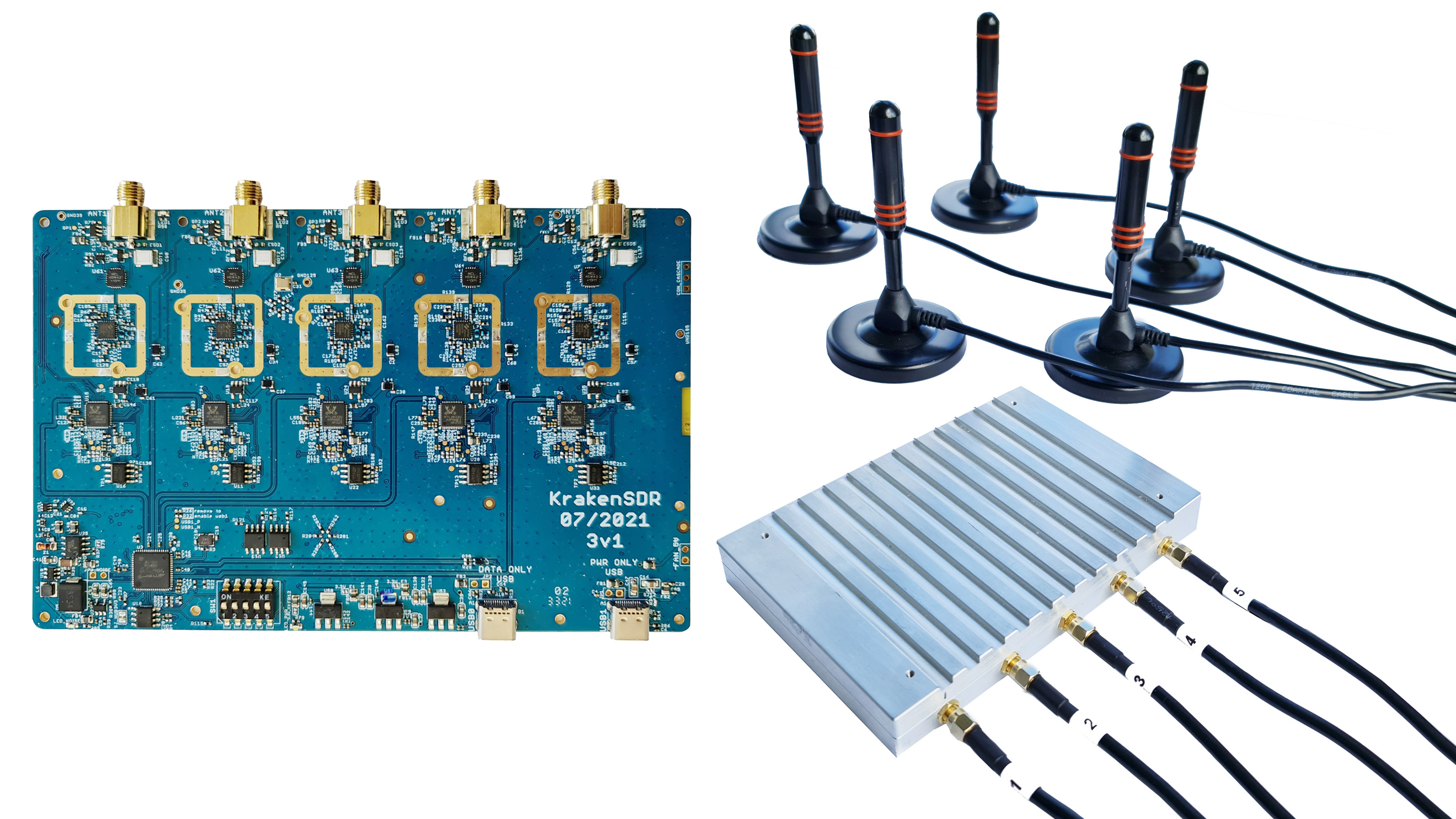
Analog phased arrays involve one phase shifter (and often one adjustable gain stage) per channel/element, implemented in analog RF circuitry. This means an analog phased array is a dedicated piece of hardware that must go alongside an SDR, or be purpose-built for a specific application. On the other hand, any SDR that contains more than one channel can be used as a digital array with no extra hardware, as long as the channels are phase coherent and sampled using the same clock, which is typically the case for SDRs that have multiple receive channels onboard. There are many SDRs that contain two receive channels, such as the Ettus USRP B210 and Analog Devices Pluto (the 2nd channel is exposed using a uFL connector on the board itself). Unfortunately, going beyond two channels involves entering the $10k+ segment of SDRs, at least as of 2023, such as the Ettus USRP N310 or the Analog Devices QuadMXFE (16 channels). The main challenge is that low-cost SDRs are typically not able to be “chained” together to scale the number of channels. The exception is the KerberosSDR (4 channels) and KrakenSDR (5 channels) which use multiple RTL-SDRs sharing an LO to form a low-cost digital array; the downside being the very limited sample rate (up to 2.56 MHz) and tuning range (up to 1766 MHz). The KrakenSDR board and example antenna configuration is shown below.

In this chapter we don’t use any specific SDRs; instead we simulate the receiving of signals using Python, and then go through the DSP used to perform beamforming/DOA for digital arrays.

Intro to Matrix Math in Python/NumPy¶

Python has many advantages over MATLAB, such as being free and open-source, diversity of applications, vibrant community, indices start from 0 like every other language, use within AI/ML, and there seems to be a library for anything you can think of. But where it falls short is how matrix manipulation is coded/represented (computationally/speed-wise, it’s plenty fast, with functions implemented under the hood efficiently in C/C++). It doesn’t help that there are multiple ways to represent matrices in Python, with the np.matrix method being deprecated in favor of np.ndarray. In this section we provide a brief primer on doing matrix math in Python using NumPy, so that when we get to the DOA examples you’ll be more comfortable.

Let’s start by jumping into the most annoying part of matrix math in NumPy; vectors are treated as 1D arrays, so there’s no way to distinguish between a row vector and column vector (it will be treated as a row vector by default), whereas in MATLAB a vector is a 2D object. In Python you can create a new vector using a = np.array([2,3,4,5]) or turn a list into a vector using mylist = [2, 3, 4, 5] then a = np.asarray(mylist), but as soon as you want to do any matrix math, orientation matters, and these will be interpreted as row vectors. Trying to do a transpose on this vector, e.g. using a.T, will not change it to a column vector! The way to make a column vector out of a normal vector a is to use a = a.reshape(-1,1). The -1 tells NumPy to figure out the size of this dimension automatically, while keeping the second dimension length 1. What this creates is technically a 2D array but the second dimension is length 1, so it’s still essentially 1D from a math perspective. It’s only one extra line, but it can really throw off the flow of matrix math code.

Now for a quick example of matrix math in Python; we will multiply a 3x10 matrix with a 10x1 matrix. Remember that 10x1 means 10 rows and 1 column, known as a column vector because it is just one column. From our early school years we know this is a valid matrix multiplication because the inner dimensions match, and the resulting matrix size is the outer dimensions, or 3x1. We will use np.random.randn() to create the 3x10 and np.arange() to create the 10x1, for convenience:

A = np.random.randn(3,10) # 3x10
B = np.arange(10) # 1D array of length 10
B = B.reshape(-1,1) # 10x1
C = A @ B # matrix multiply
print(C.shape) # 3x1
C = C.squeeze() # see next subsection
print(C.shape) # 1D array of length 3, easier for plotting and other non-matrix Python code

After performing matrix math you may find your result looks something like: [[ 0. 0.125 0.251 -0.376 -0.251 ...]] which clearly has just one dimension of data, but if you go to plot it you will either get an error or a plot that doesn’t show anything. This is because the result is technically a 2D array, and you need to convert it to a 1D array using a.squeeze(). The squeeze() function removes any dimensions of length 1, and comes in handy when doing matrix math in Python. In the example given above, the result would be [ 0. 0.125 0.251 -0.376 -0.251 ...] (notice the missing second brackets), which can be plotted or used in other Python code that expects something 1D.

When coding matrix math the best sanity check you can do is print out the dimensions (using A.shape) to verify they are what you expect. Consider sticking the shape in the comments after each line for future reference, and so it’s easy to make sure dimensions match when doing matrix or elementwise multiplication.

Here are some common operations in both MATLAB and Python, as a sort of cheat sheet to reference:

Operation	MATLAB	Python/NumPy
Create (Row) Vector, size `1 x 4`	`a = [2 3 4 5];`	`a = np.array([2,3,4,5])`
Create Column Vector, size `4 x 1`	`a = [2; 3; 4; 5];` or `a = [2 3 4 5].'`	`a = np.array([[2],[3],[4],[5]])` or `a = np.array([2,3,4,5])` then `a = a.reshape(-1,1)`
Create 2D Matrix	`A = [1 2; 3 4; 5 6];`	`A = np.array([[1,2],[3,4],[5,6]])`
Get Size	`size(A)`	`A.shape`
Transpose a.k.a. $A^T$	`A.'`	`A.T`
Complex Conjugate Transpose a.k.a. Conjugate Transpose a.k.a. Hermitian Transpose a.k.a. $A^H$	`A'`	`A.conj().T` (unfortunately there is no `A.H` for ndarrays)
Elementwise Multiply	`A .* B`	`A * B` or `np.multiply(a,b)`
Matrix Multiply	`A * B`	`A @ B` or `np.matmul(A,B)`
Dot Product of two vectors (1D)	`dot(a,b)`	`np.dot(a,b)` (never use np.dot for 2D)
Concatenate	`[A A]`	`np.concatenate((A,A))`

Steering Vector¶

To get to the fun part we have to get through a little bit of math, but the following section has been written so that the math is relatively straightforward and has diagrams to go along with it, only the most basic trig and exponential properties are used. It’s important to understand the basic math behind what we’ll do in Python to perform DOA.

Consider a 1D three-element uniformly spaced array:

Diagram showing direction of arrival (DOA) of a signal impinging on a uniformly spaced antenna array, showing boresight angle and distance between elements or apertures

In this example a signal is coming in from the right side, so it’s hitting the right-most element first. Let’s calculate the delay between when the signal hits that first element and when it reaches the next element. We can do this by forming the following trig problem, try to visualize how this triangle was formed from the diagram above. The segment highlighted in red represents the distance the signal has to travel after it has reached the first element, before it hits the next one.

Trig associated with direction of arrival (DOA) of uniformly spaced array

If you recall SOH CAH TOA, in this case we are interested in the “adjacent” side and we have the length of the hypotenuse ( $d$ ), so we need to use a cosine:

$\cos(90 - \theta) = \frac{\mathrm{adjacent}}{\mathrm{hypotenuse}}$

We must solve for adjacent, as that is what will tell us how far the signal must travel between hitting the first and second element, so it becomes adjacent $= d \cos(90 - \theta)$ . Now there is a trig identity that lets us convert this to adjacent $= d \sin(\theta)$ . This is just a distance though, we need to convert this to a time, using the speed of light: time elapsed $= d \sin(\theta) / c$ seconds. This equation applies between any adjacent elements of our array, although we can multiply the whole thing by an integer to calculate between non-adjacent elements since they are uniformly spaced (we’ll do this later).

Now to connect this trig and speed of light math to the signal processing world. Let’s denote our transmit signal at baseband $x(t)$ and it’s being transmitting at some carrier, $f_c$ , so the transmit signal is $x(t) e^{2j \pi f_c t}$ . We’ll use $d_m$ to refer to antenna spacing in meters. Lets say this signal hits the first element at time $t = 0$ , which means it hits the next element after $d_m \sin(\theta) / c$ seconds, like we calculated above. This means the 2nd element receives:

$x(t - \Delta t) e^{2j \pi f_c (t - \Delta t)}$

$\mathrm{where} \quad \Delta t = d_m \sin(\theta) / c$

recall that when you have a time shift, it is subtracted from the time argument.

When the receiver or SDR does the downconversion process to receive the signal, its essentially multiplying it by the carrier but in the reverse direction, so after doing downconversion the receiver sees:

$x(t - \Delta t) e^{2j \pi f_c (t - \Delta t)} e^{-2j \pi f_c t}$

$= x(t - \Delta t) e^{-2j \pi f_c \Delta t}$

Now we can do a little trick to simplify this even further; consider how when we sample a signal it can be modeled by substituting $t$ for $nT$ where $T$ is sample period and $n$ is just 0, 1, 2, 3… Substituting this in we get $x(nT - \Delta t) e^{-2j \pi f_c \Delta t}$ . Well, $nT$ is so much greater than $\Delta t$ that we can get rid of the first $\Delta t$ term and we are left with $x(nT) e^{-2j \pi f_c \Delta t}$ . If the sample rate ever gets fast enough to approach the speed of light over a tiny distance, we can revisit this, but remember that our sample rate only needs to be a bit larger than the signal of interest’s bandwidth.

Let’s keep going with this math but we’ll start representing things in discrete terms so that it will better resemble our Python code. The last equation can be represented as the following, let’s plug back in $\Delta t$ :

$x[n] e^{-2j \pi f_c \Delta t}$

$= x[n] e^{-2j \pi f_c d_m \sin(\theta) / c}$

We’re almost done, but luckily there’s one more simplification we can make. Recall the relationship between center frequency and wavelength: $\lambda = \frac{c}{f_c}$ , or inversely, $f_c = \frac{c}{\lambda}$ . Plugging this in we get:

$x[n] e^{-2j \pi d_m \sin(\theta) / \lambda}$

In applied beamforming and DOA we like to represent $d$ , the distance between adjacent elements, as a fraction of wavelength (instead of meters). The most common value chosen for $d$ during the array design process is to use half the wavelength. Regardless of what $d$ is, from this point on we’re going to represent $d$ as a fraction of wavelength instead of meters, making the equations and all our code simpler. I.e., $d$ (without the subscript $m$ ) represents normalized distance, and is equal to $d = d_m / \lambda$ . This means we can simplify the equation above to:

$x[n] e^{-2j \pi d \sin(\theta)}$

The above equation is specific to adjacent elements, for the signal received by the $k$ ’th element we just need to multiply $d$ times $k$ :

$x[n] e^{-2j \pi d k \sin(\theta)}$

We can represent this in matrix form by simply arranging the above equation for all Nr elements in the array, from $k = 0, 1, ... , N-1$ :

$x \begin{bmatrix} e^{-2j \pi d (0) \sin(\theta)} \\ e^{-2j \pi d (1) \sin(\theta)} \\ e^{-2j \pi d (2) \sin(\theta)} \\ \vdots \\ e^{-2j \pi d (N_r - 1) \sin(\theta)} \\ \end{bmatrix}$

where $x$ is the 1D row vector containing the transmit signal, and the column vector written out is what we call the “steering vector” (often denoted as $s$ and in code s) and represent it as an array, a 1D array for a 1D antenna array, etc. Because $e^{0} = 1$ , the first element of the steering vector is always 1, and the rest are phase shifts relative to the first element:

$s = \begin{bmatrix} 1 \\ e^{-2j \pi d (1) \sin(\theta)} \\ e^{-2j \pi d (2) \sin(\theta)} \\ \vdots \\ e^{-2j \pi d (N_r - 1) \sin(\theta)} \\ \end{bmatrix}$

And we’re done! This vector above is what you’ll see in DOA papers and ULA implementations everywhere! You may also see it with the $2\pi\sin(\theta)$ expressed as a symbol like $\psi$ , in which case the steering vector would be just $e^{-jd\psi}$ , which is the more general form (we won’t be using that form, however). In python s is:

s = [np.exp(-2j*np.pi*d*0*np.sin(theta)), np.exp(-2j*np.pi*d*1*np.sin(theta)), np.exp(-2j*np.pi*d*2*np.sin(theta)), ...] # note the increasing k
# or
s = np.exp(-2j * np.pi * d * np.arange(Nr) * np.sin(theta)) # where Nr is the number of receive antenna elements

Note how element 0 results in a 1+0j (because $e^{0}=1$ ); this makes sense because everything above was relative to that first element, so it’s receiving the signal as-is without any relative phase shifts. This is purely how the math works out, in reality any element could be thought of as the reference, but as you’ll see in our math/code later on, what matters is the difference in phase/amplitude received between elements. It’s all relative.

Remember that our d is in units of wavelengths not meters!

Receiving a Signal¶

Let’s use the steering vector concept to simulate a signal arriving at an array. For a transmit signal we’ll just use a tone for now:

import numpy as np
import matplotlib.pyplot as plt

sample_rate = 1e6
N = 10000 # number of samples to simulate

# Create a tone to act as the transmitter signal
t = np.arange(N)/sample_rate # time vector
f_tone = 0.02e6
tx = np.exp(2j * np.pi * f_tone * t)

Now let’s simulate an array consisting of three omnidirectional antennas in a line, with 1/2 wavelength between adjacent ones (a.k.a. “half-wavelength spacing”). We will simulate the transmitter’s signal arriving at this array at a certain angle, theta. Understanding the steering vector s below is why we went through all that math above.

d = 0.5 # half wavelength spacing
Nr = 3
theta_degrees = 20 # direction of arrival (feel free to change this, it's arbitrary)
theta = theta_degrees / 180 * np.pi # convert to radians
s = np.exp(-2j * np.pi * d * np.arange(Nr) * np.sin(theta)) # Steering Vector
print(s) # note that it's 3 elements long, it's complex, and the first element is 1+0j

To apply the steering vector we have to do a matrix multiplication of s and tx, so first let’s convert both to 2D, using the approach we discussed earlier when we reviewed doing matrix math in Python. We’ll start off by making both into row vectors using ourarray.reshape(-1,1). We then perform the matrix multiply, indicated by the @ symbol. We also have to convert tx from a row vector to a column vector using a transpose operation (picture it rotating 90 degrees) so that the matrix multiply inner dimensions match.

s = s.reshape(-1,1) # make s a column vector
print(s.shape) # 3x1
tx = tx.reshape(1,-1) # make tx a row vector
print(tx.shape) # 1x10000

X = s @ tx # Simulate the received signal X through a matrix multiply
print(X.shape) # 3x10000.  X is now going to be a 2D array, 1D is time and 1D is the spatial dimension

At this point X is a 2D array, size 3 x 10000 because we have three array elements and 10000 samples simulated. We use uppercase X to represent the fact that it’s multiple received signals combined (stacked) together. We can pull out each individual signal and plot the first 200 samples; below we’ll plot the real part only, but there’s also an imaginary part, like any baseband signal. One annoying part of matrix math in Python is needing to add the .squeeze(), which removes all dimensions with length 1, to get it back to a normal 1D NumPy array that plotting and other operations expects.

plt.plot(np.asarray(X[0,:]).squeeze().real[0:200]) # the asarray and squeeze are just annoyances we have to do because we came from a matrix
plt.plot(np.asarray(X[1,:]).squeeze().real[0:200])
plt.plot(np.asarray(X[2,:]).squeeze().real[0:200])
plt.show()

Note the phase shifts between elements like we expect to happen (unless the signal arrives at boresight in which case it will reach all elements at the same time and there won’t be a shift, set theta to 0 to see). Element 0 appears to arrive first, with the others slightly delayed. Try adjusting the angle and see what happens.

As one final step, let’s add noise to this received signal, as every signal we will deal with has some amount of noise. We want to apply the noise after the steering vector is applied, because each element experiences an independent noise signal (we can do this because AWGN with a phase shift applied is still AWGN):

n = np.random.randn(Nr, N) + 1j*np.random.randn(Nr, N)
X = X + 0.5*n # X and n are both 3x10000

../_images/doa_time_domain_with_noise.svg

Conventional Beamforming & DOA¶

We will now process these samples X, pretending we don’t know the angle of arrival, and perform DOA, which involves estimating the angle of arrival(s) with DSP and some Python code! As discussed earlier in this chapter, the act of beamforming and performing DOA are very similar and are often built off the same techniques. Throughout the rest of this chapter we will investigate different “beamformers”, and for each one we will start with the beamformer math/code that calculates the weights, $w$ . These weights can be “applied” to the incoming signal X through the simple equation $w^H X$ , or in Python w.conj().T @ X. In the example above, X is a 3x10000 matrix, but after we apply the weights we are left with 1x10000, as if our receiver only had one antenna, and we can use normal RF DSP to process the signal. After developing the beamformer, we will apply that beamformer to the DOA problem.

We’ll start with the “conventional” beamforming approach, a.k.a. delay-and-sum beamforming. Our weights vector w needs to be a 1D array for a uniform linear array, in our example of three elements, w is a 3x1 array of complex weights. With conventional beamforming we leave the magnitude of the weights at 1, and adjust the phases so that the signal constructively adds up in the direction of our desired signal, which we will refer to as $\theta$ . It turns out that this is the exact same math we did above, i.e., our weights are our steering vector!

$w_{conv} = e^{-2j \pi d k \sin(\theta)}$

or in Python:

w = np.exp(-2j * np.pi * d * np.arange(Nr) * np.sin(theta)) # Conventional, aka delay-and-sum, beamformer
X_weighted = w.conj().T @ X # example of applying the weights to the received signal (i.e., perform the beamforming)
print(X_weighted.shape) # 1x10000

where Nr is the number of elements in our uniform linear array with spacing of d fractions of wavelength (most often ~0.5). As you can see, the weights don’t depend on anything other than the array geometry and the angle of interest. If our array involved calibrating the phase, we would include those calibration values too. You may have been able to notice by the equation for w that the weights are complex valued and the magnitudes are all equal to one (unity).

But how do we know the angle of interest theta? We must start by performing DOA, which involves scanning through (sampling) all directions of arrival from -π to +π (-180 to +180 degrees), e.g., in 1 degree increments. At each direction we calculate the weights using a beamformer; we will start by using the conventional beamformer. Applying the weights to our signal X will give us a 1D array of samples, as if we received it with 1 directional antenna. We can then calculate the power in the signal by taking the variance with np.var(), and repeat for every angle in our scan. We will plot the results and look at it with our human eyes/brain, but what most RF DSP does is find the angle of maximum power (with a peak-finding algorithm) and call it the DOA estimate.

theta_scan = np.linspace(-1*np.pi, np.pi, 1000) # 1000 different thetas between -180 and +180 degrees
results = []
for theta_i in theta_scan:
   w = np.exp(-2j * np.pi * d * np.arange(Nr) * np.sin(theta_i)) # Conventional, aka delay-and-sum, beamformer
   X_weighted = w.conj().T @ X # apply our weights. remember X is 3x10000
   results.append(10*np.log10(np.var(X_weighted))) # power in signal, in dB so its easier to see small and large lobes at the same time
results -= np.max(results) # normalize (optional)

# print angle that gave us the max value
print(theta_scan[np.argmax(results)] * 180 / np.pi) # 19.99999999999998

plt.plot(theta_scan*180/np.pi, results) # lets plot angle in degrees
plt.xlabel("Theta [Degrees]")
plt.ylabel("DOA Metric")
plt.grid()
plt.show()

../_images/doa_conventional_beamformer.svg

We found our signal! You’re probably starting to realize where the term electrically steered array comes in. Try increasing the amount of noise to push it to its limit, you might need to simulate more samples being received for low SNRs. Also try changing the direction of arrival.

If you prefer viewing the DOA results on a polar plot, use the following code:

fig, ax = plt.subplots(subplot_kw={'projection': 'polar'})
ax.plot(theta_scan, results) # MAKE SURE TO USE RADIAN FOR POLAR
ax.set_theta_zero_location('N') # make 0 degrees point up
ax.set_theta_direction(-1) # increase clockwise
ax.set_rlabel_position(55)  # Move grid labels away from other labels
plt.show()

We will keep seeing this pattern of looping over angles, and having some method of calculating the beamforming weights, then applying them to the received signal. In the next beamforming method (MVDR) we will use our received signal X as part of the weight calculations, making it an adaptive technique. But first we will investigate some interesting things that happen with phased arrays, including why we have that second peak at 160 degrees.

180-Degree Ambiguity¶

Let’s talk about why is there a second peak at 160 degrees; the DOA we simulated was 20 degrees, but it is not a coincidence that 180 - 20 = 160. Picture three omnidirectional antennas in a line placed on a table. The array’s boresight is 90 degrees to the axis of the array, as labeled in the first diagram in this chapter. Now imagine the transmitter in front of the antennas, also on the (very large) table, such that its signal arrives at a +20 degree angle from boresight. Well the array sees the same effect whether the signal is arriving with respect to its front or back, the phase delay is the same, as depicted below with the array elements in red and the two possible transmitter DOA’s in green. Therefore, when we perform the DOA algorithm, there will always be a 180-degree ambiguity like this, the only way around it is to have a 2D array, or a second 1D array positioned at any other angle w.r.t the first array. You may be wondering if this means we might as well only calculate -90 to +90 degrees to save compute cycles, and you would be correct!

Let’s try sweeping the angle of arrival (AoA) from -90 to +90 degrees instead of keeping it constant at 20:

Animation of direction of arrival (DOA) showing the endfire of the array

As we approach the endfire of the array, which is when the signal arrives at or near the axis of the array, performance drops. We see two main degradations: 1) the main lobe gets wider and 2) we get ambiguity and don’t know whether the signal is coming from the left or the right. This ambiguity adds to the 180-degree ambiguity discussed earlier, where we get an extra lobe at 180 - theta, causing certain AoA to lead to three lobes of roughly equal size. This endfire ambiguity makes sense though, the phase shifts that occur between elements are identical whether the signal arrives from the left or right side w.r.t. the array axis. Just like with the 180-degree ambiguity, the solution is to use a 2D array or two 1D arrays at different angles. In general, beamforming works best when the angle is closer to the boresight.

From this point on, we will only be displaying -90 to +90 degrees in our polar plots, as the pattern will always be mirrored over the axis of the array, at least for 1D linear arrays (which is all we cover in this chapter).

Beam Pattern¶

The plots we have shown so far are DOA results; they correspond to the received power at each angle after applying the beamformer. They were specific to a scenario that involved transmitters arriving from certain angles. But we can also take a look at the beam pattern itself, before receiving any signal, this is sometimes referred to as the “quiescent antenna pattern” or “array response”.

Recall that our steering vector we keep seeing,

np.exp(-2j * np.pi * d * np.arange(Nr) * np.sin(theta))

encapsulates the ULA geometry, and its only other parameter is the direction you want to steer towards. We can calculate and plot the quiescent antenna pattern (array response) when steered towards a certain direction, which will tell us the arrays natural response if we don’t do any additional beamforming. This can be done by taking the FFT of the complex conjugated weights, no for loop needed! The tricky part is padding to increase resolution, and mapping the bins of the FFT output to angle in radians or degrees, which involves an arcsine as you can see in the full example below:

Nr = 3
d = 0.5
N_fft = 512
theta_degrees = 20 # there is no SOI, we arent processing samples, this is just the direction we want to point at
theta = theta_degrees / 180 * np.pi
w = np.exp(-2j * np.pi * d * np.arange(Nr) * np.sin(theta)) # conventional beamformer
w = np.conj(w) # or else our answer will be negative/inverted
w_padded = np.concatenate((w, np.zeros(N_fft - Nr))) # zero pad to N_fft elements to get more resolution in the FFT
w_fft_dB = 10*np.log10(np.abs(np.fft.fftshift(np.fft.fft(w_padded)))**2) # magnitude of fft in dB
w_fft_dB -= np.max(w_fft_dB) # normalize to 0 dB at peak

# Map the FFT bins to angles in radians
theta_bins = np.arcsin(np.linspace(-1, 1, N_fft)) # in radians

# find max so we can add it to plot
theta_max = theta_bins[np.argmax(w_fft_dB)]

fig, ax = plt.subplots(subplot_kw={'projection': 'polar'})
ax.plot(theta_bins, w_fft_dB) # MAKE SURE TO USE RADIAN FOR POLAR
ax.plot([theta_max], [np.max(w_fft_dB)],'ro')
ax.text(theta_max - 0.1, np.max(w_fft_dB) - 4, np.round(theta_max * 180 / np.pi))
ax.set_theta_zero_location('N') # make 0 degrees point up
ax.set_theta_direction(-1) # increase clockwise
ax.set_rlabel_position(55)  # Move grid labels away from other labels
ax.set_thetamin(-90) # only show top half
ax.set_thetamax(90)
ax.set_ylim([-30, 1]) # because there's no noise, only go down 30 dB
plt.show()

It turns out that this pattern is going to almost exactly match the pattern you get when performing DOA with the conventional beamformer (delay-and-sum), when there is a single tone present at theta_degrees and little-to-no noise. The plot may look different because of how low the y-axis gets in dB, or due to the size of the FFT used to create this quiescent response pattern. Try tweaking theta_degrees or the number of elements Nr to see how the response changes.

Just for fun, the following animation shows the beam pattern of the conventional beamformer, for an 8-element array being steered between -90 and +90 degrees. Also shown are the eight weights plotted in the complex plane (real and imaginary axis).

Beam pattern of delay and sum while viewing each weight on the complex plane

Note how all weights have unity magnitude (they stay on the unit circle), and how the higher numbered elements “spin” faster. If you watch closely you’ll notice at 0 degrees they all line up; they are all equal to 0 phase shift (1+0j).

Array Beamwidth¶

For those curious, there are equations that approximate the main lobe beamwidth given the number of elements, although they only work well when the number of elements is high (e.g., 8 or higher). The half power beamwidth (HPBW) is defined as the width 3 dB down from the main lobe peak, and is roughly $\frac{0.9 \lambda}{N_rd\cos(\theta)}$ [1], which for half-wavelength spacing simplifies to:

$\text{HPBW} \approx \frac{1.8}{N_r\cos(\theta)} \text{ [radians]} \qquad \text{when } d = \lambda/2$

First null beamwidth (FNBW), the width of the main lobe from null-to-null, is roughly $\frac{2\lambda}{N_rd}$ [1], which for half-wavelength spacing simplifies to:

$\text{FNBW} \approx \frac{4}{N_r} \text{ [radians]} \qquad \text{when } d = \lambda/2$

Let’s use the previous code but increase Nr to 16 elements. Using the equations above, the HPBW when pointed at 20 degrees (0.35 radians) should be roughly 0.12 radians or 6.8 degrees. The FNBW should be roughly 0.25 radians or 14.3 degrees. Let’s simulate things to see how close we are. For viewing beamwidths we tend to use rectangular plots instead of polar. Below shows the results with HPBW annotated in green and FNBW in red:

It may be hard to see in the plot, but zooming way in, we find that the HPBW is about 6.8 degrees and the FNBW is about 15.4 degrees, so pretty close to our calculations, especially HPBW!

When d is not λ/2¶

So far we have been using a distance between elements, d, equal to one half wavelength. So for example, an array designed for 2.4 GHz WiFi with λ/2 spacing would have a spacing of 3e8/2.4e9/2 = 12.5cm or about 5 inches, meaning a 4x4 element array would be about 15” x 15” x the height of the antennas. There are times when an array may not be able to achieve exactly λ/2 spacing, such as when space is restricted, or when the same array has to work on a variety of carrier frequencies.

Let’s examine when the spacing is greater than λ/2, i.e., too much spacing, by varying d between λ/2 and 4λ. We will remove the bottom half of the polar plot since it’s a mirror of the top anyway.

Animation of direction of arrival (DOA) showing what happens when distance d is much more than half-wavelength

As you can see, in addition to the 180-degree ambiguity we discussed earlier, we now have additional ambiguity, and it gets worse as d gets higher (extra/incorrect lobes form). These extra lobes are known as grating lobes, and they are a result of “spatial aliasing”. As we learned in the IQ Sampling chapter, when we don’t sample fast enough we get aliasing. The same thing happens in the spatial domain; if our elements are not spaced close enough together w.r.t. the carrier frequency of the signal being observed, we get garbage results in our analysis. You can think of spacing out antennas as sampling space! In this example we can see that the grating lobes don’t get too problematic until d > λ, but they will occur as soon as you go above λ/2 spacing. This is because Nyquist says we need to sample at least twice as fast as the signal we are observing, i.e., two samples per cycle. We measure our spatial sampling rate in samples per meter, and because the equivalent of radian frequency in space is 2π/λ radians per meter, and knowing there are 2π radians (360 degrees) in one cycle, we must sample space at least:

$\text{spatial sampling rate} \geq 2 \text{ [samples/cycle]} \cdot \frac{2\pi/\lambda \text{ [radians/meter]}}{2\pi \text{ [radians/cycle]}} \text{spatial sampling rate} \geq 2/\lambda \text{ [samples/meter]}$

or in terms of distance between elements, $d$ , which is essentially meters per spatial sample:

$d \leq \lambda/2$

As long as $d \leq \lambda/2$ we won’t have any grating lobes!

Now what happens when d is less than λ/2, such as when we need to fit the array in a small space? We know we won’t have grating lobes, but something else does happen… Let’s repeat the same simulation but start at 0.5λ and lower $d$ :

Animation of direction of arrival (DOA) showing what happens when distance d is much less than half-wavelength

While the main lobe gets wider as d gets lower, it still has a maximum at 20 degrees, and there are no grating lobes, so in theory this would still work (at least at high SNR). To better understand what breaks as d gets too small, let’s repeat the experiment but with an additional signal arriving from -40 degrees:

Animation of direction of arrival (DOA) showing what happens when distance d is much less than half-wavelength and there are two signals present

Once we get lower than λ/4 there is no distinguishing between the two different paths, and the array performs poorly. As we will see later in this chapter, there are beamforming techniques that provide more precise beams than conventional beamforming, but keeping d as close to λ/2 as possible will continue to be a theme.

Number of Elements¶

Coming soon!

Spatial Tapering¶

Spatial tapering is a technique used alongside the conventional beamformer, where the magnitude of the weights are adjusted to achieve certain features. Although even if you aren’t using the conventional beamformer, the concept of tapering is still important to understand. Recall that when we calculated the conventional beamformer weights, it was a series of complex numbers which all had magnitudes of one (unity). With spatial tapering we will multiply the weights by scalars to scale their magnitude. Let’s start by seeing what happens if we multiply the weights by random values between 0 and 1, i.e.:

tapering = np.random.uniform(0, 1, Nr) # random tapering
w *= tapering

We will simulate a signal being received at boresight (0 degrees) at high SNR to see what happens. Note that this process is equivalent and will have the same results as simulated the quiescent antenna pattern for the given weights, as we discuss at the end of this chapter.

Spatial tapering using random values to adjust the magnitude of the weights

Try to observe the width of the main lobe, and the position of nulls.

It turns out that tapering can reduce the sidelobes, which is often desired, by reducing the magnitude of the weights at the edges of the array. For example, a Hamming window function can be used as the tapering values as follows:

tapering = np.hamming(Nr) # Hamming window function
w *= tapering

Just for fun we will transition between using a rectangular window (no window) and a Hamming window, as our tapering function:

Spatial tapering using a hamming window to adjust the magnitude of the weights

We notice a couple changes here. First, the main lobe width can be made wider or narrower depending on the tapering function used (less sidelobes usually leads to a wider mainlobe). A rectangular taper (i.e., no taper) will lead to the most narrow main lobe but highest sidelobes. The second thing we notice is that the gain of the main lobe decreases when we apply a taper, and this is because we’re ultimately receiving less signal energy by not using the entire gain of all elements, which can be a major downside in very low SNR situations.

If you are curious why there are so many sidelobes when we use a rectangular window (no tapering), it is the same reason why a rectangular window in the time domain leads to spectral leakage in the frequency domain. The Fourier transform of a rectangular window is a sinc function, $sin(x)/x$ , which has sidelobes that extend to infinity. With arrays we are performing sampling in the spatial domain, and the beam pattern is the Fourier transform of that spatial sampling process combined with the weights, which is why we were able to plot the beam patter using an FFT earlier in this chapter. Recall from the Windowing Section in the Frequency Domain chapter, we compared the frequency response of each window type:

Manually Changing Weights¶

The conventional beamformer provides us an equation to calculate the weights in order to point at a specific direction, but for a moment let’s act like we don’t have any method of calculating weights, and instead we will play around with the weights (both magnitude and phase) manually to see what happens. Below is a little app written in JavaScript to simulate the beam pattern of an 8-element array, with sliders to control gain and phase of each element. You can try adding tapering, or simulating less than 8 elements by zeroing out the magnitude of one or more.

Element Magnitude (Gain) Phase

Adaptive Beamforming¶

The conventional beamformer we discussed earlier is a simple and effective way to perform beamforming, but it has some limitations. For example, it doesn’t work well when there are multiple signals arriving from different directions, or when the noise level is high. In these cases, we need to use more advanced beamforming techniques, which are often referred to as “adaptive” beamforming. The idea behind adaptive beamforming is to use the received signal to calculate the weights, instead of using a fixed set of weights like we did with the conventional beamformer. This allows the beamformer to adapt to the environment and provide better performance, because the weights are now based on the statistics of the received data.

Adaptive beamforming techniques can be further broken down into regular and subspace-based. Subspace methods such as MUSIC and ESPRIT are very powerful, but they require guessing how many signals are present, and they require at least three elements to function (although it is recommended to have at least four).

The first adaptive beamforming technique we will investigate is MVDR, which tends to be the de facto algorithm when people talk about adaptive beamforming.

MVDR/Capon Beamformer¶

We will now look at a beamformer that is slightly more complicated than the conventional/delay-and-sum technique, but tends to perform much better, called the Minimum Variance Distortionless Response (MVDR) or Capon Beamformer. Recall that variance of a signal corresponds to how much power is in the signal. The idea behind MVDR is to keep the signal at the angle of interest at a fixed gain of 1 (0 dB), while minimizing the total variance/power of the resulting beamformed signal. If our signal of interest is kept fixed then minimizing the total power means minimizing interferers and noise as much as possible. It is often referred to as a “statistically optimal” beamformer.

The MVDR/Capon beamformer can be summarized in the following equation:

$w_{mvdr} = \frac{R^{-1} s}{s^H R^{-1} s}$

The vector $s$ is the steering vector corresponding to the desired direction and was discussed at the beginning of this chapter. $R$ is the spatial covariance matrix estimate based on our received samples, found using R = np.cov(X) or calculated manually by multiplying X with the complex conjugate transpose of itself, i.e., $R = X X^H$ , The spatial covariance matrix is a Nr x Nr size matrix (3x3 in the examples we have seen so far) that tells us how similar the samples received from the three elements are. While this equation may seem confusing at first, it helps to know that the denominator is mainly there for scaling, and the numerator is the important part to focus on, which is just the inverted covariance matrix multiplied by the steering vector. That being said, we still need to include the denominator, it acts as a normalizing constant so that as $R$ changes over time, the weights don’t change in magnitude.

For those interested in the MVDR derivation, expand this

Beamforming Output - The output of the beamformer using a weight vector $\mathbf{w}$ is given by:

$y(t) = \mathbf{w}^H \mathbf{x}(t)$

Optimization Problem - The goal is to determine the beamforming weights that minimize the output power subject to a distortion-less response towards a desired direction $\theta_0$ . Formally, the problem can be expressed as:

$\min_{\mathbf{w}} \, \mathbf{w}^H \mathbf{R} \mathbf{w} \quad \text{subject to} \quad \mathbf{w}^H \mathbf{s} = 1$

where:

$\mathbf{R} = E[\mathbf{X}\mathbf{X}^H]$ is the covariance matrix of the received signals
$\mathbf{s}$ is the steering vector towards the desired signal direction $\theta_0$

Lagrangian Method - Introduce a Lagrange multiplier $\lambda$ and form the Lagrangian:

$L(\mathbf{w}, \lambda) = \mathbf{w}^H \mathbf{R} \mathbf{w} - \lambda (\mathbf{w}^H \mathbf{s} - 1)$

Solving the Optimization - Differentiating the Lagrangian with respect to the $\mathbf{w^H}$ and setting the derivative to zero, we obtain:

$\frac{\partial L}{\partial \mathbf{w}^*} = 2\mathbf{R}\mathbf{w} - \lambda \mathbf{s} = 0 \mathbf{w} = \lambda \mathbf{s} \mathbf{{R^{-1}}}$

To solve for $\lambda$ , apply the constraint $\mathbf{w}^H \mathbf{s} = 1$ :

$\implies (\lambda \mathbf{s^{H}}\mathbf{{R^{-1}}})s = 1 \implies \lambda = \frac{1}{\mathbf{s}^{H}\mathbf{R}^{-1}\mathbf{s}} \mathbf{R}\mathbf{w} = \lambda \mathbf{s} \mathbf{w_{mvdr}} = \frac{\mathbf{R}^{-1} \mathbf{s}}{\mathbf{s}^H \mathbf{R}^{-1} \mathbf{s}}$

If we already know the direction of the signal of interest, and that direction does not change, we only have to calculate the weights once and simply use them to receive our signal of interest. Although even if the direction doesn’t change, we benefit from recalculating these weights periodically, to account for changes in the interference/noise, which is why we refer to these non-conventional digital beamformers as “adaptive” beamforming; they use information in the signal we receive to calculate the best weights. Just as a reminder, we can perform beamforming using MVDR by calculating these weights and applying them to the signal with w.conj().T @ X, just like we did in the conventional method, the only difference is how the weights are calculated.

To perform DOA using the MVDR beamformer, we simply repeat the MVDR calculation while scanning through all angles of interest. I.e., we act like our signal is coming from angle $\theta$ , even if it isn’t. At each angle we calculate the MVDR weights, then apply them to the received signal, then calculate the power in the signal. The angle that gives us the highest power is our DOA estimate, or even better we can plot power as a function of angle to see the beam pattern, as we did above with the conventional beamformer, that way we don’t need to assume how many signals are present.

In Python we can implement the MVDR/Capon beamformer as follows, which will be done as a function so that it’s easy to use later on:

# theta is the direction of interest, in radians, and X is our received signal
def w_mvdr(theta, r):
   s = np.exp(-2j * np.pi * d * np.arange(Nr) * np.sin(theta)) # steering vector in the desired direction theta
   s = s.reshape(-1,1) # make into a column vector (size 3x1)
   R = (X @ X.conj().T)/X.shape[1] # Calc covariance matrix. gives a Nr x Nr covariance matrix of the samples
   Rinv = np.linalg.pinv(R) # 3x3. pseudo-inverse tends to work better/faster than a true inverse
   w = (Rinv @ s)/(s.conj().T @ Rinv @ s) # MVDR/Capon equation! numerator is 3x3 * 3x1, denominator is 1x3 * 3x3 * 3x1, resulting in a 3x1 weights vector
   return w

Using this MVDR beamformer in the context of DOA, we get the following Python example:

theta_scan = np.linspace(-1*np.pi, np.pi, 1000) # 1000 different thetas between -180 and +180 degrees
results = []
for theta_i in theta_scan:
   w = w_mvdr(theta_i, r) # 3x1
   X_weighted = w.conj().T @ X # apply weights
   power_dB = 10*np.log10(np.var(X_weighted)) # power in signal, in dB so its easier to see small and large lobes at the same time
   results.append(power_dB)
results -= np.max(results) # normalize

When applied to the previous DOA example simulation, we get the following:

It appears to work fine, but to really compare this to other techniques we’ll have to create a more interesting problem. Let’s set up a simulation with an 8-element array receiving three signals from different angles: 20, 25, and 40 degrees, with the 40 degree one received at a much lower power than the other two, as a way to spice things up. Our goal will be to detect all three signals, meaning we want to be able to see noticeable peaks (high enough for a peak-finder algorithm to extract). The code to generate this new scenario is as follows:

Nr = 8 # 8 elements
theta1 = 20 / 180 * np.pi # convert to radians
theta2 = 25 / 180 * np.pi
theta3 = -40 / 180 * np.pi
s1 = np.exp(-2j * np.pi * d * np.arange(Nr) * np.sin(theta1)).reshape(-1,1) # 8x1
s2 = np.exp(-2j * np.pi * d * np.arange(Nr) * np.sin(theta2)).reshape(-1,1)
s3 = np.exp(-2j * np.pi * d * np.arange(Nr) * np.sin(theta3)).reshape(-1,1)
# we'll use 3 different frequencies.  1xN
tone1 = np.exp(2j*np.pi*0.01e6*t).reshape(1,-1)
tone2 = np.exp(2j*np.pi*0.02e6*t).reshape(1,-1)
tone3 = np.exp(2j*np.pi*0.03e6*t).reshape(1,-1)
X = s1 @ tone1 + s2 @ tone2 + 0.1 * s3 @ tone3 # note the last one is 1/10th the power
n = np.random.randn(Nr, N) + 1j*np.random.randn(Nr, N)
X = X + 0.05*n # 8xN

You can put this code at the top of your script, since we are generating a different signal than the original example. If we run our MVDR beamformer on this new scenario we get the following results:

It works pretty well, we can see the two signals received only 5 degrees apart, and we can also see the 3rd signal (at -40 or 320 degrees) that was received at one tenth the power of the others. Now let’s run the conventional beamformer on this new scenario:

While it might be a pretty shape, it’s not finding all three signals at all… By comparing these two results we can see the benefit from using a more complex and “adaptive” beamformer.

As a quick aside for the interested reader, there is actually an optimization that can be made when performing DOA with MVDR, using a trick. Recall that we calculate the power in a signal by taking the variance, which is the mean of the magnitude squared (assuming our signals average value is zero which is almost always the case for baseband RF). We can represent taking the power in our signal after applying our weights as:

$P_{mvdr} = \frac{1}{N} \sum_{n=0}^{N-1} \left| w^H_{mvdr} r_n \right|^2$

If we switch from using a summation to the expectation operator, and plug in the equation for the MVDR weights, we get:

$P_{mvdr} = E \left( \left| w^H_{mvdr} X_n \right| ^2 \right) = w^H_{mvdr} E \left( X X^H \right) w_{mvdr} = w^H_{mvdr} R w_{mvdr} = \frac{s^H R^{-1} s}{s^H R^{-1} s} \cdot R \cdot \frac{R^{-1} s}{s^H R^{-1} s} = \frac{s^H R^{-1} s}{(s^H R^{-1} s)(s^H R^{-1} s)} = \frac{1}{s^H R^{-1} s}$

Meaning we don’t have to apply the weights at all, this final equation above for power can be used directly in our DOA scan, saving us some computations:

def power_mvdr(theta, r):
    s = np.exp(-2j * np.pi * d * np.arange(r.shape[0]) * np.sin(theta)) # steering vector in the desired direction theta_i
    s = s.reshape(-1,1) # make into a column vector (size 3x1)
    R = (X @ X.conj().T)/X.shape[1] # Calc covariance matrix. gives a Nr x Nr covariance matrix of the samples
    Rinv = np.linalg.pinv(R) # 3x3. pseudo-inverse tends to work better than a true inverse
    return 1/(s.conj().T @ Rinv @ s).squeeze()

To use this in the previous simulation, within the for loop, the only thing left to do is take the 10*np.log10() and you’re done, there are no weights to apply; we skipped calculating the weights!

There are many more beamformers out there, but next we are going to take a moment to discuss how the number of elements impacts our ability to perform beamforming and DOA.

Covariance Matrix¶

Let’s take a brief moment to discuss the spatial covariance matrix, which is a key concept in adaptive beamforming. A covariance matrix is a mathematical representation of the similarity between pairs of elements in a random vector (in our case, it’s the elements in our array, so we call it the spatial covariance matrix). A covariance matrix is always square, and the values along the diagonal correspond to the covariance of each element with itself. We calculate the spatial covariance matrix estimate; it is only an estimate because we have a limited number of samples.

In general, the covariance matrix is defined as:

$\mathrm{cov}(X) = E \left[ (X - E[X])(X - E[X])^H \right]$

for wireless signals at baseband, $E[X]$ is typically zero or very close to zero, so this simplifies to:

$\mathrm{cov}(X) = E[X X^H]$

Given a limited number of IQ samples, $\bm{X}$ , we can estimate this covariance, which we will denote as $\hat{R}$ :

$\hat{R} = \frac{\bm{X} \bm{X}^H}{N} = \frac{1}{N} \sum^N_{n=1} X_n X_n^H$

where $N$ is the number of samples (not the number of elements). In Python this looks like:

R = (X @ X.conj().T)/X.shape[1]

Alternatively, we can use the built-in NumPy function:

R = np.cov(X)

As an example, we will look at the spatial covariance matrix for the scenario where we only had one transmitter and three elements:

[[ 1.494+0.j    0.486+0.881j -0.543+0.839j]
 [ 0.486-0.881j 1.517 +0.j    0.483+0.886j]
 [-0.543-0.839j 0.483-0.886j  1.499+0.j   ]]

Note how the diagonal elements are real and roughly the same, this is because they are really only telling us the received signal power at each element, which will be roughly the same between elements since they are all set to the same gain. The off-diagonal elements are really where the important values are, although looking at the raw values doesn’t tell us much other than there is a significant amount of correlation between elements.

As part of adaptive beamforming you will see a pattern where we take the inverse of the spatial correlation matrix. This inverse tells us how two elements are related to each other after removing the influence of other elements. It is referred to as the “precision matrix” in statistics and “whitening matrix” in radar.

LCMV Beamformer¶

While MVDR is powerful, what if we have more than one SOI? Thankfully, with just a small tweak to MVDR, we can implement a scheme that handles multiple SOIs, called the Linearly Constrained Minimum Variance (LCMV) beamformer. It is a generalization of MVDR, where we specify the desired response for multiple directions, kind of like a spatial version of SciPy’s firwin2() for those familiar with it. The optimum weight vector for the LCMV beamformer can be summarized in the following equation:

$w_{lcmv} = R^{-1} C [C^H R^{-1} C]^{-1} f$

where $C$ is a matrix comprising of the steering vectors of the corresponding SOIs and interferers, and $f$ is the desired response vector. The vector $f$ for a particular row takes the value of 0 when the corresponding steering vector is to be nulled, and takes a value of 1 when we want a beam pointed at it. For example, if we have two sources of interest and two sources of interference, we can set f = [1,1,0,0]. The LCMV beamformer is a powerful tool that can be used to suppress interference and noise from multiple directions while simultaneously enhancing the signal of interest from multiple directions. The catch is that the total number of nulls and beams you can form simultaneously is limited by the size of the array (the number of elements). Furthermore, you need to craft the steering vector for each of the SOIs and interferers, which isn’t always readily available in practical applications. When estimates are used instead, the performance of the LCMV beamformer can degrade. It is for this reason that we prefer to steer nulls using the spatial covariance matrix $R$ (based on statistics of the received signal), instead of “hardcoding” nulls by estimating the AoA of the interferer (which could have error) and crafting the steering vector in that direction, with a 0 added to $f$ .

As far as performing LCMV in Python, it is very similar to MVDR, but we have to specify C which is made up of potentially multiple steering vectors, and f which is a 1D array of 1’s and 0’s as previously mentioned. The following code snippet demonstrates how to implement the LCMV beamformer for two SOIs (15 and 60 degrees); recall that MVDR only supports 1 SOI at a time. Therefore, our f = [1; 1] with no zeros, as we will not be including any “hardcoded” nulls. We will simulate a scenario with four interferers, arriving from angles -60, -30, 0, and 30 degrees.

# Let's point at the SOI at 15 deg, and another potential SOI that we didn't actually simulate at 60 deg
soi1_theta = 15 / 180 * np.pi # convert to radians
soi2_theta = 60 / 180 * np.pi

# LCMV weights
R_inv = np.linalg.pinv(np.cov(X)) # 8x8
s1 = np.exp(-2j * np.pi * d * np.arange(Nr) * np.sin(soi1_theta)).reshape(-1,1) # 8x1
s2 = np.exp(-2j * np.pi * d * np.arange(Nr) * np.sin(soi2_theta)).reshape(-1,1) # 8x1
C = np.concatenate((s1, s2), axis=1) # 8x2
f = np.ones(2).reshape(-1,1) # 2x1

# LCMV equation
#    8x8   8x2                    2x8        8x8   8x2  2x1
w = R_inv @ C @ np.linalg.pinv(C.conj().T @ R_inv @ C) @ f # output is 8x1

We can plot the beam pattern of w using the FFT method we showed earlier:

Example beam pattern when using the LCMV beamformer

As you can see, we have beams pointed at the two directions of interest, and nulls at the locations of the interferers (like MVDR, we don’t have to tell it where the emitters are, it figures it out based on the received signal). Green and red dots are added to the plot to show AoAs of the SOIs and interferers, respectively.

For the full code expand this section

# Simulate received signal
Nr = 8 # 8 elements
theta1 = -60 / 180 * np.pi # convert to radians
theta2 = -30 / 180 * np.pi
theta3 = 0 / 180 * np.pi
theta4 = 30 / 180 * np.pi
s1 = np.exp(-2j * np.pi * d * np.arange(Nr) * np.sin(theta1)).reshape(-1,1) # 8x1
s2 = np.exp(-2j * np.pi * d * np.arange(Nr) * np.sin(theta2)).reshape(-1,1)
s3 = np.exp(-2j * np.pi * d * np.arange(Nr) * np.sin(theta3)).reshape(-1,1)
s4 = np.exp(-2j * np.pi * d * np.arange(Nr) * np.sin(theta4)).reshape(-1,1)
# we'll use 3 different frequencies.  1xN
tone1 = np.exp(2j*np.pi*0.01e6*t).reshape(1,-1)
tone2 = np.exp(2j*np.pi*0.02e6*t).reshape(1,-1)
tone3 = np.exp(2j*np.pi*0.03e6*t).reshape(1,-1)
tone4 = np.exp(2j*np.pi*0.04e6*t).reshape(1,-1)
X = s1 @ tone1 + s2 @ tone2 + s3 @ tone3 + s4 @ tone4
n = np.random.randn(Nr, N) + 1j*np.random.randn(Nr, N)
X = X + 0.5*n # 8xN

# Let's point at the SOI at 15 deg, and another potential SOI that we didn't actually simulate at 60 deg
soi1_theta = 15 / 180 * np.pi # convert to radians
soi2_theta = 60 / 180 * np.pi

# LCMV weights
R_inv = np.linalg.pinv(np.cov(X)) # 8x8
s1 = np.exp(-2j * np.pi * d * np.arange(Nr) * np.sin(soi1_theta)).reshape(-1,1) # 8x1
s2 = np.exp(-2j * np.pi * d * np.arange(Nr) * np.sin(soi2_theta)).reshape(-1,1) # 8x1
C = np.concatenate((s1, s2), axis=1) # 8x2
f = np.ones(2).reshape(-1,1) # 2x1

# LCMV equation
#    8x8   8x2                    2x8        8x8   8x2  2x1
w = R_inv @ C @ np.linalg.pinv(C.conj().T @ R_inv @ C) @ f # output is 8x1

# Plot beam pattern
w = w.squeeze() # reduce to a 1D array
N_fft = 1024
w = np.conj(w) # or else our answer will be negative/inverted
w_padded = np.concatenate((w, np.zeros(N_fft - Nr))) # zero pad to N_fft elements to get more resolution in the FFT
w_fft_dB = 10*np.log10(np.abs(np.fft.fftshift(np.fft.fft(w_padded)))**2) # magnitude of fft in dB
w_fft_dB -= np.max(w_fft_dB) # normalize to 0 dB at peak
theta_bins = np.arcsin(np.linspace(-1, 1, N_fft)) # Map the FFT bins to angles in radians

fig, ax = plt.subplots(subplot_kw={'projection': 'polar'})
ax.plot(theta_bins, w_fft_dB) # MAKE SURE TO USE RADIAN FOR POLAR
# Add dots where interferers and SOIs are
ax.plot([theta1], [0], 'or')
ax.plot([theta2], [0], 'or')
ax.plot([theta3], [0], 'or')
ax.plot([theta4], [0], 'or')
ax.plot([soi1_theta], [0], 'og')
ax.plot([soi2_theta], [0], 'og')
ax.set_theta_zero_location('N') # make 0 degrees point up
ax.set_theta_direction(-1) # increase clockwise
ax.set_thetagrids(np.arange(-90, 105, 15)) # it's in degrees
ax.set_rlabel_position(55)  # Move grid labels away from other labels
ax.set_thetamin(-90) # only show top half
ax.set_thetamax(90)
ax.set_ylim([-30, 1]) # because there's no noise, only go down 30 dB
plt.show()

There is a special use-case of LCMV that you may have already thought of; let’s say instead of pointing the main beam at exactly 20 degrees, for example, you want a beam wider than what the conventional beamformer would normally provide. You can do this by setting the desired response vector f to be a vector of 1’s over a range of angles (e.g., several values from 10 to 30 degrees), and zeros elsewhere. This is a powerful tool that can be used to create a beam pattern that is wider than the main lobe of the conventional beamformer, which is always a plus in real-world scenarios where the exact angle of arrival is not known. The same approach can be used to create a null at a specific direction, spread out over a relatively wide range of angles. Just remember that doing this will use several degrees of freedom! As an example of this approach, let’s simulate an 18-element array and point the angle of interest from 15 to 30 degrees using 4 different thetas, and a null from 45 to 60 degrees using 4 different thetas. We won’t simulate any actual interferers.

Nr = 18
X = np.random.randn(Nr, N) + 1j*np.random.randn(Nr, N) # Simulate received signal of just noise

# Let's point at the SOI from 15 to 30 degrees using 4 different thetas
soi_thetas = np.linspace(15, 30, 4) / 180 * np.pi # convert to radians

# Let's make a null from 45 to 60 degrees using 4 different thetas
null_thetas = np.linspace(45, 60, 4) / 180 * np.pi # convert to radians

# LCMV weights
R_inv = np.linalg.pinv(np.cov(X))
s = []
for soi_theta in soi_thetas:
    s.append(np.exp(-2j * np.pi * d * np.arange(Nr) * np.sin(soi_theta)).reshape(-1,1))
for null_theta in null_thetas:
    s.append(np.exp(-2j * np.pi * d * np.arange(Nr) * np.sin(null_theta)).reshape(-1,1))
C = np.concatenate(s, axis=1)
f = np.asarray([1]*len(soi_thetas) + [0]*len(null_thetas)).reshape(-1,1)
w = R_inv @ C @ np.linalg.pinv(C.conj().T @ R_inv @ C) @ f # LCMV equation

# Plot beam pattern as before...

Example beam pattern when using the LCMV beamformer with a spread beam and a spread null

The beam and null is spread out over the range we requested! Try changing the number of thetas for the main beam and/or the null, as well as the number of elements, to see if the resulting weights are able to satisfy the desired response.

Null Steering¶

Now that we’ve seen LCMV, it is worth investigating a simpler technique that can be used in both analog and digital arrays, called null steering. Think of it like an extension to the conventional beamformer, but in addition to pointing a beam at the direction of interest, we can also place nulls at specific angles. This technique does not involve changing the weights based on the received signal (e.g., we never calculate R), and thus is not considered adaptive. In the simulation below, we don’t even need to simulate a signal, we can simply craft the weights of our beamformer using null steering to place nulls at predefined angles, then visualize the beam pattern.

The weights for null steering are calculated by starting with the conventional beamformer pointed at the direction of interest, and then we use the sidelobe-canceler equation to update the weights to include the nulls, one null at a time. The sidelobe-canceler equation is:

$w_{\text{new}} = w_{\text{orig}} - \frac{w_{\text{null}}^H w_{\text{orig}}}{w_{\text{null}}^H w_{\text{null}}} w_{\text{null}}$

where $w_{\text{null}}$ is the steering vector in the direction of the null we want to add to $w_{\text{orig}}$ . The weights are updated by subtracting the scaled null steering vector from the current weights. The scaling factor is calculated by projecting the current weights onto the null steering vector, and dividing by the projection of the null steering vector onto itself. This is then repeated for each null direction ( $w_{\text{orig}}$ starts as the conventional beamforming weights but then gets updated after each null is added). The full process looks like:

$\text{1:} \qquad w_{\text{orig}} = e^{-2j \pi d k \sin(\theta_{SOI})} \qquad \text{2:} \qquad w_{\text{null}} = e^{-2j \pi d k \sin(\theta_{null})} \qquad \text{3:} \qquad w_{\text{new}} = w_{\text{orig}} - \frac{w_{\text{null}}^H w_{\text{orig}}}{w_{\text{null}}^H w_{\text{null}}} w_{\text{null}} \text{4:} \qquad w_{\text{orig}} = w_{\text{new}} \qquad \qquad \qquad \text{5:} \qquad \text{GOTO 2 to add next null}$

Let’s simulate an 8-element array, and place four nulls:

d = 0.5
Nr = 8

theta_soi = 30 / 180 * np.pi # convert to radians
nulls_deg = [-60, -30, 0, 60] # degrees
nulls_rad = np.asarray(nulls_deg) / 180 * np.pi

# Start out with conventional beamformer pointed at theta_soi
w = np.exp(-2j * np.pi * d * np.arange(Nr) * np.sin(theta_soi)).reshape(-1,1)

# Loop through nulls
for null_rad in nulls_rad:
    # weights equal to steering vector in target null direction
    w_null = np.exp(-2j * np.pi * d * np.arange(Nr) * np.sin(null_rad)).reshape(-1,1)

    # scaling_factor (complex scalar) for w at nulled direction
    scaling_factor = w_null.conj().T @ w / (w_null.conj().T @ w_null)
    print("scaling_factor:", scaling_factor, scaling_factor.shape)

    # Update weights to include the null
    w = w - w_null @ scaling_factor # sidelobe-canceler equation

# Plot beam pattern
N_fft = 1024
w = np.conj(w) # or else our answer will be negative/inverted
w_padded = np.concatenate((w.squeeze(), np.zeros(N_fft - Nr))) # zero pad to N_fft elements to get more resolution in the FFT
w_fft_dB = 10*np.log10(np.abs(np.fft.fftshift(np.fft.fft(w_padded)))**2) # magnitude of fft in dB
w_fft_dB -= np.max(w_fft_dB) # normalize to 0 dB at peak
theta_bins = np.arcsin(np.linspace(-1, 1, N_fft)) # Map the FFT bins to angles in radians

fig, ax = plt.subplots(subplot_kw={'projection': 'polar'})
ax.plot(theta_bins, w_fft_dB)
# Add dots where nulls and SOI are
for null_rad in nulls_rad:
    ax.plot([null_rad], [0], 'or')
ax.plot([theta_soi], [0], 'og')
ax.set_theta_zero_location('N') # make 0 degrees point up
ax.set_theta_direction(-1) # increase clockwise
ax.set_thetagrids(np.arange(-90, 105, 15)) # it's in degrees
ax.set_rlabel_position(55) # Move grid labels away from other labels
ax.set_thetamin(-90) # only show top half
ax.set_thetamax(90)
ax.set_ylim([-40, 1]) # because there's no noise, only go down -40 dB
plt.show()

We get the following beam pattern. You may notice nulls in positions that you did not request; that is intended and a result of the limited number of elements. You may also find that with too few elements, you either don’t have nulls/beam exactly where you intend, or it may not be able to fit the criteria at all due to a lack of degrees of freedom (number of elements minus 1).

MUSIC¶

We will now change gears and talk about a different kind of beamformer. All of the previous ones have fallen in the “delay-and-sum” category, but now we will dive into “sub-space” methods. These involve dividing the signal subspace and noise subspace, which means we must estimate how many signals are being received by the array, to get a good result. MUltiple SIgnal Classification (MUSIC) is a very popular sub-space method that involves calculating the eigenvectors of the covariance matrix (which is a computationally intensive operation by the way). We split the eigenvectors into two groups: signal sub-space and noise-subspace, then project steering vectors into the noise sub-space and steer for nulls. That might seem confusing at first, which is part of why MUSIC seems like black magic!

The core MUSIC equation is the following:

$\hat{\theta} = \mathrm{argmax}\left(\frac{1}{s^H V_n V^H_n s}\right)$

where $V_n$ is that list of noise sub-space eigenvectors we mentioned (a 2D matrix). It is found by first calculating the eigenvectors of $R$ , which is done simply by w, v = np.linalg.eig(R) in Python, and then splitting up the vectors (w) based on how many signals we think the array is receiving. There is a trick for estimating the number of signals that we’ll talk about later, but it must be between 1 and Nr - 1. I.e., if you are designing an array, when you are choosing the number of elements you must have one more than the number of anticipated signals. One thing to note about the equation above is $V_n$ does not depend on the steering vector $s$ , so we can precalculate it before we start looping through theta. The full MUSIC code is as follows:

num_expected_signals = 3 # Try changing this!

# part that doesn't change with theta_i
R = np.cov(X) # Calc covariance matrix. gives a Nr x Nr covariance matrix
w, v = np.linalg.eig(R) # eigenvalue decomposition, v[:,i] is the eigenvector corresponding to the eigenvalue w[i]
eig_val_order = np.argsort(np.abs(w)) # find order of magnitude of eigenvalues
v = v[:, eig_val_order] # sort eigenvectors using this order
# We make a new eigenvector matrix representing the "noise subspace", it's just the rest of the eigenvalues
V = np.zeros((Nr, Nr - num_expected_signals), dtype=np.complex64)
for i in range(Nr - num_expected_signals):
   V[:, i] = v[:, i]

theta_scan = np.linspace(-1*np.pi, np.pi, 1000) # -180 to +180 degrees
results = []
for theta_i in theta_scan:
    s = np.exp(-2j * np.pi * d * np.arange(Nr) * np.sin(theta_i)) # Steering Vector
    s = s.reshape(-1,1)
    metric = 1 / (s.conj().T @ V @ V.conj().T @ s) # The main MUSIC equation
    metric = np.abs(metric.squeeze()) # take magnitude
    metric = 10*np.log10(metric) # convert to dB
    results.append(metric)

results /= np.max(results) # normalize

Running this algorithm on the complex scenario we have been using, we get the following very precise results, showing the power of MUSIC:

Example of direction of arrival (DOA) using MUSIC algorithm beamforming

Now what if we had no idea how many signals were present? Well there is a trick; you sort the eigenvalue magnitudes from highest to lowest, and plot them (it may help to plot them in dB):

plot(10*np.log10(np.abs(w)),'.-')

The eigenvalues associated with the noise-subspace are going to be the smallest, and they will all tend around the same value, so we can treat these low values like a “noise floor”, and any eigenvalue above the noise floor represents a signal. Here we can clearly see there are three signals being received, and adjust our MUSIC algorithm accordingly. If you don’t have a lot of IQ samples to process or the signals are at low SNR, the number of signals might not be as obvious. Feel free to play around by adjusting num_expected_signals between 1 and 7, you’ll find that underestimating the number will lead to missing signal(s) while overestimating will only slightly hurt performance.

Another experiment worth trying with MUSIC is to see how close two signals can arrive at (in angle) while still distinguishing between them; sub-space techniques are especially good at that. The animation below shows an example, with one signal at 18 degrees and another slowly sweeping angle of arrival.

ESPRIT¶

Coming soon!

Circular Arrays¶

We will briefly talk about the Uniform Circular Array (UCA), which is a popular array geometry for DOA because it gets around the 180-degree ambiguity issue ULAs have. The KrakenSDR, for example, is a 5-element array, and it is common to place those five elements in a circle with equal spacing between elements. In theory, only three elements is needed to form a UCA, just like how we can make a ULA with only two elements.

All of the code we have studied so far applies to UCAs, we just have to replace the steering vector equation with one specific to the UCA:

radius = 0.05 # normalized by wavelength!
d = np.sqrt(2 * radius**2 * (1 - np.cos(2*np.pi/Nr)))
sf = 1.0 / (np.sqrt(2.0) * np.sqrt(1.0 - np.cos(2*np.pi/Nr))) # scaling factor based on geometry, eg for a hexagon it is 1.0
x = d * sf * np.cos(2 * np.pi / Nr * np.arange(Nr))
y = -1 * d * sf * np.sin(2 * np.pi / Nr * np.arange(Nr))
s = np.exp(1j * 2 * np.pi * (x * np.cos(theta) + y * np.sin(theta)))
s = s.reshape(-1, 1) # Nrx1

Lastly, you will want to scan from 0 to 360 degrees, instead of just -90 to +90 degrees like with a ULA.

Training Data¶

Within the context of array processing, there is a concept of “training”, where you establish the covariance matrix R before the potential SOI is present. This is especially used in radar, where most of the time, there is no SOI present, and the entire detection process is about testing a series of angles to check if there is a SOI present. When we calculate R before the SOI is present, it lets us calculate weights using methods like MVDR with only the interferers and noise environment encapsulated in the covariance matrix. That way there is no chance that MVDR decides to put a null at or near the direction of the SOI. We then use the weights and apply them to the received signal to test whether the SOI is now present at that angle.

To demonstrate the value of using training data, we will perform MVDR on a recording taken from an actual 16-element array (using the QUAD-MxFE platform from Analog Devices). We will start by performing MVDR as usual, with the entire received signal being used to calculate R and the weights. We will then use a separate recording which was taken before the SOI was turned on, to calculate R and the weights.

These recordings were taken at an RF frequency of 3.3 GHz, with an array using a 0.045 meter spacing, so d is 0.495. A 30 MHz sample rate was used. We will refer to the three signals as A, B, and C. Signal C will be the designated SOI, while A and B will be interferers. Therefore, we need a recording with just A and B in order to create the training data, without A and B moving between taking the training data and the recording that includes C. Below are links to the two recordings you will need:

https://github.com/777arc/777arc.github.io/raw/master/3p3G_A_B.npy

https://github.com/777arc/777arc.github.io/raw/master/3p3G_A_B_C.npy

Let’s start by performing normal MVDR with the A_B_C recording. We can load in the recording, which is a np.save() format containing a 2D array, with the first dimension being the number of elements in the array, and the second dimension being the number of samples:

import matplotlib.pyplot as plt
import numpy as np

# Array params
center_freq = 3.3e9
sample_rate = 30e6
d = 0.045 * center_freq / 3e8
print("d:", d)

# Includes all three signals, we'll call C our SOI
filename = '3p3G_A_B_C.npy'
X = np.load(filename)
Nr = X.shape[0]

Next we will perform basic DOA with MVDR, to identify the angles of arrival of the three signals:

# Perform DOA to find angle of arrival of C
theta_scan = np.linspace(-1*np.pi/2, np.pi/2, 10000) # between -90 and +90 degrees
results = []
R = X @ X.conj().T # Calc covariance matrix. gives a Nr x Nr covariance matrix of the samples
Rinv = np.linalg.pinv(R) # pseudo-inverse tends to work better than a true inverse
for theta_i in theta_scan:
   a = np.exp(-2j * np.pi * d * np.arange(X.shape[0]) * np.sin(theta_i)) # steering vector in the desired direction theta_i
   a = a.reshape(-1,1) # make into a column vector
   power = 1/(a.conj().T @ Rinv @ a).squeeze() # MVDR power equation
   power_dB = 10*np.log10(np.abs(power)) # power in signal, in dB so its easier to see small and large lobes at the same time
   results.append(power_dB)
results -= np.max(results) # normalize to 0 dB at peak

This is one of those situations where it’s easier to just use a rectangular plot instead of polar. We have labeled the signals A, B, and C.

Next, if we want to call C our SOI, and use MVDR to create weights that will null out A and B and preserve C, we need to know the exact angle of arrival of C. We will do this using an argmax on the DOA results we just created above, but only after zeroing out the angles corresponding to A and B (we do this by setting the upper 60% of our DOA results to very very low value).

# Pull out angle of C, after zeroing out the angles that include the interferers
results_temp = np.array(results)
results_temp[int(len(results)*0.4):] = -9999*np.ones(int(len(results)*0.6))
max_angle = theta_scan[np.argmax(results_temp)] # radians
print("max_angle:", max_angle)

It turns out that C is arriving at -0.3407 radians, so that is what we need to use when calculating our MVDR weights. You have done this many times, it’s just the MVDR equation:

# Calc MVDR weights
s = np.exp(-2j * np.pi * d * np.arange(Nr) * np.sin(max_angle)) # steering vector in the desired direction theta
s = s.reshape(-1,1) # make into a column vector
w = (Rinv @ s)/(s.conj().T @ Rinv @ s) # MVDR/Capon equation

Lastly, let’s plot the beam pattern of the MVDR weights we just calculated, as well as the DOA results we had earlier, and a dashed green line at max_angle:

Expand this for the plotting code (it's nothing new)

# Calc beam pattern
w = np.conj(w.squeeze()) # or else our answer will be negative/inverted
N_fft = 2048
w_padded = np.concatenate((w, np.zeros(N_fft - Nr))) # zero pad to N_fft elements to get more resolution in the FFT
w_fft_dB = 10*np.log10(np.abs(np.fft.fftshift(np.fft.fft(w_padded)))**2) # magnitude of fft in dB
w_fft_dB -= np.max(w_fft_dB) # normalize to 0 dB at peak
theta_bins = np.arcsin(np.linspace(-1, 1, N_fft)) # Map the FFT bins to angles in radians

# Plot beam pattern and DOA results
plt.plot(theta_bins * 180 / np.pi, w_fft_dB) # MAKE SURE TO USE RADIAN FOR POLAR
plt.plot(theta_scan * 180 / np.pi, results, 'r')
plt.vlines(ymax=np.max(results), ymin=np.min(results) , x=max_angle*180/np.pi, color='g', linestyle='--')
plt.xlabel("Angle [deg]")
plt.ylabel("Magnitude [dB]")
plt.title("Beam Pattern and DOA Results, Without Training")
plt.grid()
plt.show()

DOA without training data DOA and MVDR beam pattern

We were successful at creating nulls at A and B. At the position of C (green dashed line), we don’t have a null, but we also don’t have what seems to be a “main lobe”; it’s sort of a reduced lobe. This is partially because there was little-to-no energy coming from the directions other than A, B, and C, so even though you see some lobes (e.g. around -70, 25, and 40 degrees), they don’t really matter because no signal is coming from that direction. Another reason the lobe at C isn’t as strong is because the main lobe is sort of fighting with the nulls that would have been created by MVDR if we were not pointed exactly in that direction. That being said, it would be nice to have a strong main lobe at our max_angle position, and to do that we will need to use training data.

We will now load the recording of just A and B, in order to create the training data. In a radar situation, this is equivalent of calculating R before you transmit any radar pulse (ideally, extremely shortly before).

# Load "training data" which is just A and B, then calc Rinv
filename = '3p3G_A_B.npy'
X_A_B = np.load(filename)
R_training = X_A_B @ X_A_B.conj().T # Calc covariance matrix
Rinv_training = np.linalg.pinv(R_training)

This time, the big difference is that we will use Rinv_training when calculating the MVDR weights. We will reuse max_angle that we already found. That way, we are pointing in the direction of C but not incorporating C into the received signal used when calculating R and R_inv.

# Calc MVDR weights using training Rinv
s = np.exp(-2j * np.pi * d * np.arange(Nr) * np.sin(max_angle)) # steering vector in the desired direction theta
s = s.reshape(-1,1) # make into a column vector (size 3x1)
w = (Rinv_training @ s)/(s.conj().T @ Rinv_training @ s) # MVDR/Capon equation

Using the same method of plotting, we get:

DOA with training data DOA and MVDR beam pattern

Note that we still get nulls from A and B (B’s null is less, but B is also a weaker signal), but this time there is a massive main lobe directed towards our angle of interest, C. This is the power of training data, and why it is so important in radar applications.

Conclusion and References¶

All Python code, including code used to generate the figures/animations, can be found on the textbook’s GitHub page.

DOA implementation in GNU Radio - https://github.com/EttusResearch/gr-doa
DOA implementation used by KrakenSDR - https://github.com/krakenrf/krakensdr_doa/blob/main/_signal_processing/krakenSDR_signal_processor.py

[1] Mailloux, Robert J. Phased Array Antenna Handbook. Second edition, Artech House, 2005