 Online Python Console
 One-time Donation


19. Приклад повної реалізації
У цій главі ми об’єднуємо багато концепцій, про які ми раніше вивчали, і розглядаємо повний приклад отримання та декодування справжнього цифрового сигналу. Ми розглянемо систему радіоданих (RDS), яка є комунікаційним протоколом для вбудовування невеликих обсягів інформації в FM-радіопередачі, наприклад назву станції та пісні. Нам доведеться демодулювати FM, зсув частоти, фільтрувати, знищувати, повторно дискретизувати, синхронізувати, декодувати та аналізувати байти. Зразок файлу IQ надається для тестування або якщо у вас під рукою немає SDR.
Знайомство з FM-радіо та RDS
Щоб зрозуміти RDS, ми повинні спочатку розглянути FM-радіотрансляції та структуру їх сигналів. Ви, мабуть, знайомі з аудіочастиною FM-сигналів, яка є просто аудіосигналами, частотно-модульованими та переданими на центральних частотах, що відповідають назві станції, наприклад, “WPGC 95.5 FM” центрується точно на 95,5 МГц. Крім звукової частини, кожна FM-передача містить деякі інші компоненти, частотно-модульовані разом зі звуком. Замість того, щоб просто шукати в Google структуру сигналу, давайте подивимося на спектральну щільність потужності (PSD) прикладу FM-сигналу після демодуляції FM. Ми розглядаємо лише позитивну частину, оскільки вихід FM-демодуляції є реальним сигналом, навіть якщо вхід був складним (незабаром ми переглянемо код для виконання цієї демодуляції).

Дивлячись на сигнал у частотній області, ми помічаємо такі окремі сигнали:
- Сигнал високої потужності між 0 - 17 кГц
- Тон на 19 кГц
- З центром на 38 кГц і шириною приблизно 30 кГц ми бачимо цікавий симетричний сигнал
- Сигнал у формі подвійної пелюстки з центром на 57 кГц
- Сигнал у формі однієї пелюстки з центром на 67 кГц
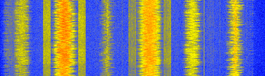
Це, по суті, все, що ми можемо визначити, просто подивившись на PSD, і пам’ятайте, що це після демодуляції FM. PSD перед демодуляцією FM виглядає наступним чином, що насправді не говорить нам багато.

Зважаючи на це, важливо розуміти, що коли ви модулюєте сигнал FM, вища частота сигналу даних призведе до вищої частоти результуючого FM-сигналу. Таким чином, присутність сигналу з центром на 67 кГц збільшує загальну смугу пропускання, яку займає переданий FM-сигнал, оскільки максимальна частотна складова зараз становить приблизно 75 кГц, як показано в першому PSD вище. Правило пропускної здатності Карсона, застосоване до FM, говорить нам, що FM-станції займають приблизно 250 кГц спектру, тому ми зазвичай виконуємо вибірку на 250 кГц (нагадаємо, що під час використання квадратурної/IQ дискретизації, ваша отримана пропускна здатність дорівнює вашій частоті дискретизації).
Швидко зазначимо, що деякі читачі, можливо, знайомі з переглядом FM-діапазону за допомогою SDR або аналізатора спектру та побаченням наступної спектрограми, і думаючи, що блокові сигнали, що знаходяться поруч із деякими FM-станціями, є RDS.
Виявляється, ці блокові сигнали насправді є HD Radio, цифровою версією того самого FM-радіосигналу (той самий аудіовміст). Ця цифрова версія забезпечує більш високу якість аудіосигналу в приймачі, оскільки аналоговий FM завжди включатиме певний шум після демодуляції, оскільки це аналогова схема, але цифровий сигнал можна демодулювати/декодувати без шуму, припускаючи, що є нульові бітові помилки.
Повернемося до п’яти сигналів, які ми виявили в нашому PSD; на наступній діаграмі показано, для чого використовується кожен сигнал.
- :: ../_images/fm_psd_labeled.svg
scale: 80 align: center alt: Компоненти FM-радіосигналу, зокрема моно- і стереозвук, RDS і сигнали DirectBand
Пройдімося по кожному з цих сигналів у довільному порядку:
Моно та стерео аудіосигнали просто переносять аудіосигнал, додавання та віднімання яких дає вам лівий та правий канали.
Пілотний тон 19 кГц використовується для демодуляції стереозвуку. Якщо ви подвоїте тон, він діятиме як опорна частота і фаза, оскільки стереозвук центрований на частоті 38 кГц. Подвоєння тону можна зробити простим піднесенням відліків до квадрата, згадайте властивість Фур’є зсуву частоти, про яку ми дізналися у розділі Частотна область.
DirectBand - це бездротова мережа передачі даних у Північній Америці, що належала та управлялася компанією Microsoft, також відома як “MSN Direct” на споживчих ринках. DirectBand передавала інформацію на такі пристрої, як портативні GPS-приймачі, наручні годинники та домашні метеостанції. Він навіть дозволяв користувачам отримувати короткі повідомлення з Windows Live Messenger. Одним з найуспішніших застосувань DirectBand було відображення даних про місцевий трафік у реальному часі на GPS-приймачах Garmin, якими користувалися мільйони людей до того, як смартфони стали повсюдним явищем. Служба DirectBand була закрита в січні 2012 року, що викликає питання, чому ми бачимо її в наших FM-сигналах, які були записані після 2012 року? Моє єдине припущення полягає в тому, що більшість FM-передавачів були спроектовані і виготовлені задовго до 2012 року, і навіть без активної “подачі” DirectBand вони все одно щось передають, можливо, пілотні символи.
Нарешті, ми підійшли до RDS, якому присвячена решта цієї глави. Як ми бачили в нашому першому PSD, смуга пропускання RDS становить приблизно 4 кГц (до того, як він отримує FM-модуляцію), і знаходиться між стереозвуком і сигналом DirectBand. Це протокол цифрового зв’язку з низькою швидкістю передачі даних, який дозволяє FM-станціям передавати разом зі звуком ідентифікацію станції, інформацію про програму, час та іншу інформацію. Стандарт RDS опублікований як стандарт IEC 62106 і може бути знайдений тут.
Сигнал RDS
У цій главі ми будемо використовувати Python для прийому RDS, але для того, щоб краще зрозуміти, як його приймати, ми повинні спочатку дізнатися про те, як формується і передається сигнал.
Передавальна сторона
RDS-інформація, яка передається FM-станцією (наприклад, назва треку тощо), кодується у набори по 8 байт. Кожен набір з 8 байт, що відповідає 64 бітам, об’єднується з 40 “контрольними бітами” в одну “групу”. Ці 104 біти передаються разом, хоча між групами немає часового проміжку, тому з точки зору одержувача, він отримує ці біти безперервно і повинен визначити межу між групами з 104 біт. Ми побачимо більше деталей про кодування і структуру повідомлень, коли зануримося в сторону прийому.
Для бездротового передавання цих бітів RDS використовує BPSK, яка, як ми дізналися з розділу Цифрова модуляція, є простою схемою цифрової модуляції, що використовується для зіставлення одиниць і нулів з фазою несучої. Як і багато протоколів на основі BPSK, RDS використовує диференціальне кодування, яке просто означає, що одиниці і нулі даних кодуються зміною одиниць і нулів, що дозволяє вам більше не перейматися тим, що ви зсунуті по фазі на 180 градусів (докладніше про це пізніше). Символи BPSK передаються зі швидкістю 1187,5 символів на секунду, а оскільки BPSK несе один біт на символ, це означає, що RDS має необроблену швидкість передачі даних приблизно 1,2 кбіт/с (включаючи накладні витрати). RDS не містить канального кодування (так званої прямої корекції помилок), хоча пакети даних містять циклічну перевірку надлишковості (CRC), щоб знати, коли сталася помилка.
Потім остаточний сигнал BPSK зсувається по частоті до 57 кГц і додається до всіх інших компонентів FM-сигналу, після чого модулюється і передається в ефір на частоті радіостанції. FM-радіосигнали передаються з надзвичайно високою потужністю порівняно з більшістю інших бездротових засобів зв’язку - до 80 кВт! Ось чому багато користувачів SDR встановлюють FM-фільтр (тобто фільтр, що обмежує смугу пропускання) в лінію з антеною; таким чином, FM не додає перешкод до того, що вони намагаються прийняти.
Хоча це був лише короткий огляд сторони передачі, ми зануримося в подробиці, коли будемо обговорювати прийом RDS.
Сторона прийому
Для того, щоб демодулювати і декодувати RDS, ми виконаємо наступні кроки, багато з яких є кроками на стороні передачі у зворотному порядку (не потрібно запам’ятовувати цей список, ми пройдемося по кожному кроку окремо нижче):
- Отримайте FM-радіосигнал, центрований на частоті станції (або прочитаний у записі IQ), зазвичай з частотою дискретизації 250 кГц
- Демодулюйте FM за допомогою так званої “квадратурної демодуляції”
- Зсув частоти на 57 кГц, щоб сигнал RDS був центрований на 0 Гц
- Фільтр низьких частот, щоб відфільтрувати все, крім RDS (також діє як узгоджений фільтр)
- Зменшити на 10, щоб ми могли працювати з меншою частотою дискретизації, оскільки ми все одно відфільтрували вищі частоти
- Передискретизуємо до 19 кГц, що дасть нам цілу кількість відліків на символ
- Синхронізація часу на рівні символів, з використанням Мюллера і Мюллера у цьому прикладі
- Точна частотна синхронізація за допомогою циклу Костаса
- Демодуляція BPSK в 1 та 0
- Диференціальне декодування, щоб скасувати застосоване диференціальне кодування
- Декодування 1 та 0 у групи байт
- Синтаксичний аналіз груп байтів у наш кінцевий результат
Хоча це може виглядати як багато кроків, RDS насправді є одним із найпростіших протоколів бездротового цифрового зв’язку. Сучасний бездротовий протокол, наприклад WiFi або 5G, потребує цілої книги, щоб охопити навіть інформацію високого рівня про рівні PHY/MAC.
Тепер ми зануримося в Python-код, який використовується для прийому RDS. Цей код був протестований із записом FM-радіо, який можна знайти тут, хоча ви можете подати і власний сигнал за умови, що він прийнятий з достатньо високим SNR: просто налаштуйтеся на центральну частоту станції та дискретизуйте зі швидкістю 250 кГц. Щоб максимізувати потужність прийнятого сигналу (наприклад, якщо ви перебуваєте в приміщенні), корисно використати напівхвильову дипольну антену належної довжини (~1,5 метра), а не 2,4 ГГц-антени, що постачаються з Pluto. Водночас FM — дуже гучний сигнал, і якщо ви біля вікна або на вулиці, антен 2,4 ГГц, ймовірно, буде достатньо, щоб прийняти сильніші радіостанції.
У цьому розділі ми будемо показувати невеликі фрагменти коду окремо, з поясненнями, але той самий код наведений наприкінці цієї глави одним великим блоком. Кожен підрозділ представить блок коду та пояснить, що він робить.
Отримання сигналу
import numpy as np
from scipy.signal import resample_poly, firwin, bilinear, lfilter
import matplotlib.pyplot as plt

# Read in signal
x = np.fromfile('/home/marc/Downloads/fm_rds_250k_1Msamples.iq', dtype=np.complex64)
sample_rate = 250e3
center_freq = 99.5e6
Ми зчитуємо наш тестовий запис, який дискретизовано на 250 кГц і центровано на FM-станції, прийнятій із високим SNR. Обов’язково оновіть шлях до файлу відповідно до вашої системи та місця збереження запису. Якщо у вас вже налаштований SDR, що працює з Python, можете приймати живий сигнал, хоча корисно спершу перевірити весь код на відомому робочому IQ-записі. Протягом цього коду ми використовуватимемо x для зберігання поточного сигналу, з яким виконуємо обробку.
FM-демодуляція
# Quadrature Demod
x = 0.5 * np.angle(x[0:-1] * np.conj(x[1:])) # see https://wiki.gnuradio.org/index.php/Quadrature_Demod
Як ми обговорювали на початку цієї глави, кілька окремих сигналів поєднуються за частотою та FM-модулюються, утворюючи те, що фактично передається в ефір. Тож перший крок — зняти цю FM-модуляцію. Іншими словами, інформація закодована у зміні частоти прийнятого сигналу, і ми хочемо демодулювати його так, щоб інформація опинилася в амплітуді, а не у частоті. Зауважте, що результат цієї демодуляції є дійсним сигналом, навіть якщо ми подавали комплексний сигнал.
Що робить цей єдиний рядок Python, так це спершу обчислює добуток нашого сигналу на затриману та спряжену версію цього сигналу. Потім він знаходить фазу кожного відліку в цьому результаті — саме в цей момент сигнал переходить від комплексного до дійсного. Щоб переконатися, що таким чином ми повертаємо інформацію, закладену у зміні частоти, розглянемо тон із частотою \(f\) та довільною фазою \(\phi\), який можна подати як \(e^{j2 \pi (f t + \phi)}\). У дискретному часі, де використовуємо цілий \(n\) замість \(t\), це стає \(e^{j2 \pi (f n + \phi)}\). Спряжена та затримана версія матиме вигляд \(e^{-j2 \pi (f (n-1) + \phi)}\). Добуток цих двох виразів дає \(e^{j2 \pi f}\), що чудово, адже \(\phi\) зникає, і коли ми обчислюємо фазу цього виразу, залишається лише \(f\).
Одним із зручних побічних ефектів FM-модуляції є те, що зміни амплітуди прийнятого сигналу не впливають на гучність аудіо, на відміну від AM-радіо.
Зсув частоти
# Freq shift
N = len(x)
f_o = -57e3 # amount we need to shift by
t = np.arange(N)/sample_rate # time vector
x = x * np.exp(2j*np.pi*f_o*t) # down shift
Далі ми зсуваємо частоту вниз на 57 кГц, використовуючи прийом \(e^{j2 \pi f_ot}\), з яким ми познайомилися в розділі Синхронізація, де f_o — це зсув частоти в герцах, а t — просто часовий вектор; те, що він починається з 0, неважливо, головне — правильний період дискретизації (обернений до частоти дискретизації). До речі, оскільки на вході ми маємо дійсний сигнал, не має значення, використаємо ми -57 чи +57 кГц, бо від’ємні частоти симетричні до додатних, тож у будь-якому випадку RDS зміститься до 0 Гц.
Фільтрація для виділення RDS
# Low-Pass Filter
taps = firwin(numtaps=101, cutoff=7.5e3, fs=sample_rate)
x = np.convolve(x, taps, 'valid')
Тепер нам потрібно відфільтрувати все, окрім RDS. Оскільки RDS ми вже вирівняли по центру 0 Гц, нам потрібен фільтр низьких частот. Ми використовуємо firwin() для синтезу FIR-фільтра (тобто обчислення коефіцієнтів), якому потрібно знати лише бажану кількість коефіцієнтів і частоту зрізу. Також слід вказати частоту дискретизації, інакше firwin не зможе правильно інтерпретувати частоту зрізу. Отриманий фільтр є симетричним ФНЧ, тож його коефіцієнти дійсні, і ми можемо застосувати його до сигналу за допомогою згортки. Ми обираємо режим 'valid', щоб позбутися крайових ефектів згортки, хоча в даному випадку це не критично, адже сигнал дуже довгий і кілька дивних відліків на краях нічого не зіпсують.
Примітка: згодом я оновлю цей фільтр на справжній узгоджений (з кореневою піднятою косинусоїдою, яку, як я вважаю, використовує RDS) задля повноти викладу, але підхід із firwin() дає ті самі показники помилок, що й коректний узгоджений фільтр у GNU Radio, тож це явно не сувора вимога.
Децимація на 10
# Decimate by 10, now that we filtered and there wont be aliasing
x = x[::10]
sample_rate = 25e3
Щоразу, коли ви відсікаєте більшу частину смуги пропускання (наприклад, ми починали зі 125 кГц реальної смуги і залишили лише 7,5 кГц), має сенс виконати децимацію. Згадайте початок розділу Вибірка IQ, де ми вчили про частоту Найквіста та можливість повністю відтворити смуговий сигнал, якщо дискретизувати принаймні з подвійною максимальною частотою. Тепер, після ФНЧ, наша максимальна частота приблизно 7,5 кГц, тож нам достатньо частоти дискретизації 15 кГц. Для запасу використаємо 25 кГц (згодом це ще й зручно з математичної точки зору).
Ми виконуємо децимацію, просто відкидаючи 9 з кожних 10 відліків, адже раніше частота дискретизації була 250 кГц, а тепер нам потрібно 25 кГц. Це може спершу збивати з пантелику, ніби ми викидаємо 90% інформації, але якщо знову перечитати розділ Вибірка IQ, ви побачите, що ми нічого не втрачаємо: ми належно відфільтрували сигнал (виконавши роль антиаліасингового фільтра) та зменшили максимальну частоту, а отже й смугу сигналу.
З погляду коду це, мабуть, найпростіший крок із усіх, але не забудьте оновити змінну sample_rate, щоб вона відображала нову частоту дискретизації.
Перевиділення до 19 кГц
# Resample to 19kHz
x = resample_poly(x, 19, 25) # up, down
sample_rate = 19e3
У розділі Pulse Shaping ми закріпили поняття “відліки на символ” і побачили зручність цілої кількості відліків на символ (дробові значення теж можливі, але працювати з ними незручно). Як уже згадувалося, RDS використовує BPSK зі швидкістю 1187,5 символів за секунду. Якщо залишити наш сигнал із частотою дискретизації 25 кГц, отримаємо 21,052631579 відліків на символ (зупиніться й перевірте обчислення, якщо це здається дивним). Отже, нам потрібна частота дискретизації, що є цілим кратним 1187,5 Гц, але не можна знижувати її надто сильно, інакше ми не “вмістимо” всю смугу сигналу. У попередньому підрозділі ми говорили, що нам потрібна частота принаймні 15 кГц, і вибрали 25 кГц для запасу.
Пошук найкращої частоти, до якої слід перевиділити, зводиться до бажаної кількості відліків на символ; працюємо у зворотному напрямку. Припустімо, що ми хочемо 10 відліків на символ. Помноживши швидкість символів RDS 1187,5 на 10, отримуємо 11,875 кГц — на жаль, цього недостатньо для Найквіста. А якщо взяти 13 відліків на символ? 1187,5 × 13 = 15 437,5 Гц — більше ніж 15 кГц, але число незручне. Наступний ступінь двійки — 16 відліків на символ. 1187,5 × 16 = рівно 19 кГц! Така “красивість” числа — це не випадковість, а особливість протоколу.
Щоб перевиділити з 25 кГц до 19 кГц, ми використовуємо resample_poly(), який спершу збільшує частоту дискретизації на цілий множник, фільтрує, а потім зменшує її на інший цілий множник. Це зручно, адже замість 25000 і 19000 можна працювати з 25 та 19. Якби ми обрали 13 відліків на символ із частотою 15 437,5 Гц, resample_poly() застосувати не вийшло б, і процес перевиділення був би значно складнішим.
І знову ж таки, не забувайте оновлювати змінну sample_rate після кожної операції, що змінює частоту дискретизації.
Синхронізація в часі (рівень символів)
# Symbol sync, using what we did in sync chapter
samples = x # for the sake of matching the sync chapter
samples_interpolated = resample_poly(samples, 32, 1) # we'll use 32 as the interpolation factor, arbitrarily chosen, seems to work better than 16
sps = 16
mu = 0.01 # initial estimate of phase of sample
out = np.zeros(len(samples) + 10, dtype=np.complex64)
out_rail = np.zeros(len(samples) + 10, dtype=np.complex64) # stores values, each iteration we need the previous 2 values plus current value
i_in = 0 # input samples index
i_out = 2 # output index (let first two outputs be 0)
while i_out < len(samples) and i_in+32 < len(samples):
    out[i_out] = samples_interpolated[i_in*32 + int(mu*32)] # grab what we think is the "best" sample
    out_rail[i_out] = int(np.real(out[i_out]) > 0) + 1j*int(np.imag(out[i_out]) > 0)
    x = (out_rail[i_out] - out_rail[i_out-2]) * np.conj(out[i_out-1])
    y = (out[i_out] - out[i_out-2]) * np.conj(out_rail[i_out-1])
    mm_val = np.real(y - x)
    mu += sps + 0.01*mm_val
    i_in += int(np.floor(mu)) # round down to nearest int since we are using it as an index
    mu = mu - np.floor(mu) # remove the integer part of mu
    i_out += 1 # increment output index
x = out[2:i_out] # remove the first two, and anything after i_out (that was never filled out)
Нарешті ми готові до синхронізації символів/часу. Тут ми використаємо той самий алгоритм синхронізації годинника Мюллера—Мюллера з розділу Синхронізація; зверніться до нього, якщо хочете краще зрозуміти принцип роботи. Кількість відліків на символ (sps) встановлюємо рівною 16, як обговорювали раніше. Значення підсилення μ = 0.01 було підібрано експериментально і працює добре. Тепер вихід має містити один відлік на символ, тобто ми отримуємо “м’які символи”, у яких може залишатися невеликий частотний зсув. Наступна анімація сузір’я дозволяє переконатися, що ми справді бачимо символи BPSK (із обертанням через частотний зсув).

Якщо ви використовуєте власний FM-сигнал і не бачите на цьому етапі двох окремих скупчень комплексних відліків, це означає або те, що синхронізація символів не спрацювала, або якась з попередніх стадій виконана некоректно. Анімація сузір’я не обов’язкова, але якщо будуєте графік, не відображайте всі відліки одразу — вони утворять суцільне коло. Побудувавши лише 100–200 відліків за раз, ви краще зрозумієте, чи справді утворюються два скупчення, навіть якщо вони обертаються.
Точна частотна синхронізація
# Fine freq sync
samples = x # for the sake of matching the sync chapter
N = len(samples)
phase = 0
freq = 0
# These next two params is what to adjust, to make the feedback loop faster or slower (which impacts stability)
alpha = 8.0
beta = 0.002
out = np.zeros(N, dtype=np.complex64)
freq_log = []
for i in range(N):
    out[i] = samples[i] * np.exp(-1j*phase) # adjust the input sample by the inverse of the estimated phase offset
    error = np.real(out[i]) * np.imag(out[i]) # This is the error formula for 2nd order Costas Loop (e.g. for BPSK)

    # Advance the loop (recalc phase and freq offset)
    freq += (beta * error)
    freq_log.append(freq * sample_rate / (2*np.pi)) # convert from angular velocity to Hz for logging
    phase += freq + (alpha * error)

    # Optional: Adjust phase so its always between 0 and 2pi, recall that phase wraps around every 2pi
    while phase >= 2*np.pi:
        phase -= 2*np.pi
    while phase < 0:
        phase += 2*np.pi
x = out
Ми також використаємо код точної частотної синхронізації з розділу Синхронізація, де застосовується цикл Костаса для усунення залишкового частотного зсуву та вирівнювання сигналу BPSK уздовж дійсної (I) осі, змушуючи компоненту Q наближатися до нуля. Якщо цикл Костаса налаштовано належним чином, усе, що залишається в Q, — це шум сигналу. Для наочності погляньмо на ту саму анімацію сузір’я після виконання частотної синхронізації (жодного обертання!).
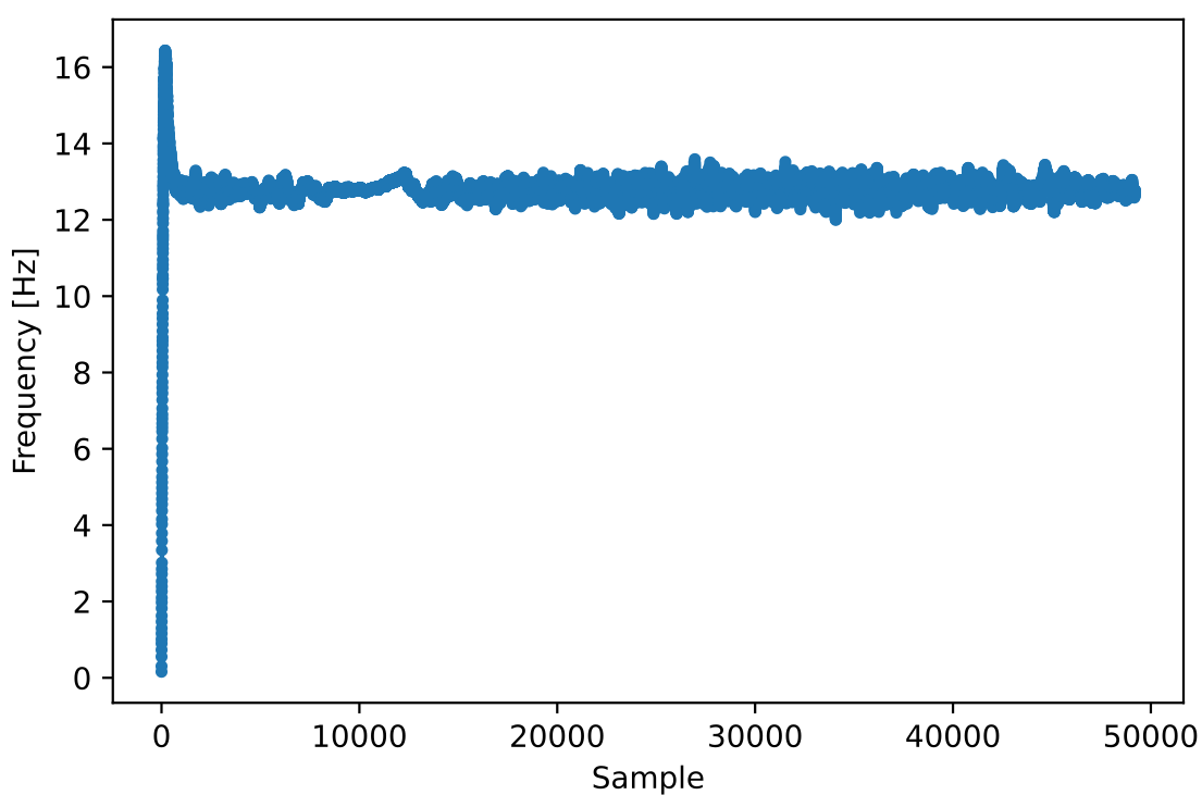
Крім того, можна подивитися на оцінку частотної помилки в часі, щоб побачити, як працює цикл Костаса; зверніть увагу, що ми зберігаємо ці дані в коді вище. Здається, залишковий зсув становив приблизно 13 Гц — або через неточність генератора передавача, або приймача (імовірніше, приймача). Якщо ви працюєте зі своїм сигналом, можливо, доведеться підлаштувати коефіцієнти alpha і beta, щоб крива виглядала подібно: синхронізація має досягатися досить швидко (наприклад, за кілька сотень символів) і підтримуватися без значних коливань. Візерунок, який ви бачите після стабілізації, — це джиттер частоти, а не коливання.
Демодуляція BPSK
# Demod BPSK
bits = (np.real(x) > 0).astype(int) # 1's and 0's
На цьому етапі демодуляція BPSK дуже проста: кожен відлік відповідає одному м’якому символу, тож нам лишається лише перевірити, чи відлік більший або менший за 0. Виклик .astype(int) дозволяє працювати з масивом цілих чисел замість булевих значень. Може виникнути питання, що саме означає значення вище чи нижче нуля — 1 чи 0. Як ми побачимо на наступному кроці, це не має значення!
Диференціальне декодування
# Differential decoding, so that it doesn't matter whether our BPSK was 180 degrees rotated without us realizing it
bits = (bits[1:] - bits[0:-1]) % 2
bits = bits.astype(np.uint8) # for decoder
Під час формування сигналу BPSK застосовувалося диференціальне кодування, тобто кожна одиниця й нуль вихідних даних перетворювалися так, що перехід з 1 у 0 або з 0 в 1 відповідав значенню 1, а відсутність зміни — значенню 0. Перевага диференціального кодування полягає в тому, що нам не потрібно хвилюватися про поворот сигналу на 180 градусів: немає значення, вважаємо ми 1 більшою чи меншою за нуль — важливим є лише факт переходу між 1 та 0. Щоб краще це відчути, подивімося на приклад нижче, який показує перші 10 символів до та після диференціального декодування:
[1 1 1 1 0 1 0 0 1 1] # before differential decoding
[- 0 0 0 1 1 1 0 1 0] # after differential decoding
Декодування RDS
Ми нарешті отримали біти інформації й готові розібратися, що вони означають! Великий блок коду нижче перетворює наші 1 та 0 на групи байтів. Було б набагато зрозуміліше, якби ми спершу створили передавальну частину RDS, але наразі достатньо знати, що байти RDS згруповані по 12: перші 8 містять дані, а останні 4 виконують роль синхрослова (так званих “offset words”). Останні 4 байти наступному кроку (парсеру) не потрібні, тому ми їх не передаємо. Цей код отримує наші 1 та 0 (масив типу uint8) і повертає список списків із 8 байтів, що зручно для наступного етапу, де ми оброблятимемо групи по 8 байтів за раз.
Більшість коду нижче присвячена синхронізації (на рівні байтів, а не символів) і перевірці помилок. Дані обробляються блоками по 104 біти: кожен блок або приймається правильно, або містить помилку (це перевіряється за допомогою CRC). Після кожних 50 блоків перевіряється, чи не було більше 35 помилкових; якщо так, усі змінні скидаються й алгоритм намагається синхронізуватися знову. CRC виконується з використанням 10-бітного полінома \(x^{10}+x^8+x^7+x^5+x^4+x^3+1\), що реалізовано як XOR регістра reg зі значенням 0x5B9 — двійковим представленням цього полінома. У Python побітові оператори [and, or, not, xor] — це & | ~ ^, як і в C++. Зсув вліво x << y дорівнює множенню на \(2^y\), а зсув вправо x >> y еквівалентний діленню на \(2^y\), також як у C++.
Зауважте, що вам не обов’язково вчитуватися в увесь цей код, особливо якщо ви зосереджені на вивченні фізичного рівня DSP/SDR, адже тут немає сигнал-обробки. Це просто реалізація декодера RDS, і практично нічого з нього не можна повторно використати для інших протоколів, настільки специфічним є сам RDS. Якщо ви вже втомилися від цієї глави, сміливо пропускайте цей величезний блок коду: він виконує відносно просте завдання, але досить громіздко.
# Constants
syndrome = [383, 14, 303, 663, 748]
offset_pos = [0, 1, 2, 3, 2]
offset_word = [252, 408, 360, 436, 848]

# see Annex B, page 64 of the standard
def calc_syndrome(x, mlen):
    reg = 0
    plen = 10
    for ii in range(mlen, 0, -1):
        reg = (reg << 1) | ((x >> (ii-1)) & 0x01)
        if (reg & (1 << plen)):
            reg = reg ^ 0x5B9
    for ii in range(plen, 0, -1):
        reg = reg << 1
        if (reg & (1 << plen)):
            reg = reg ^ 0x5B9
    return reg & ((1 << plen) - 1) # select the bottom plen bits of reg

# Initialize all the working vars we'll need during the loop
synced = False
presync = False

wrong_blocks_counter = 0
blocks_counter = 0
group_good_blocks_counter = 0

reg = np.uint32(0) # was unsigned long in C++ (64 bits) but numpy doesn't support bitwise ops of uint64, I don't think it gets that high anyway
lastseen_offset_counter = 0
lastseen_offset = 0

# the synchronization process is described in Annex C, page 66 of the standard */
bytes_out = []
for i in range(len(bits)):
    # in C++ reg doesn't get init so it will be random at first, for ours its 0s
    # It was also an unsigned long but never seemed to get anywhere near the max value
    # bits are either 0 or 1
    reg = np.bitwise_or(np.left_shift(reg, 1), bits[i]) # reg contains the last 26 rds bits. these are both bitwise ops
    if not synced:
        reg_syndrome = calc_syndrome(reg, 26)
        for j in range(5):
            if reg_syndrome == syndrome[j]:
                if not presync:
                    lastseen_offset = j
                    lastseen_offset_counter = i
                    presync = True
                else:
                    if offset_pos[lastseen_offset] >= offset_pos[j]:
                        block_distance = offset_pos[j] + 4 - offset_pos[lastseen_offset]
                    else:
                        block_distance = offset_pos[j] - offset_pos[lastseen_offset]
                    if (block_distance*26) != (i - lastseen_offset_counter):
                        presync = False
                    else:
                        print('Sync State Detected')
                        wrong_blocks_counter = 0
                        blocks_counter = 0
                        block_bit_counter = 0
                        block_number = (j + 1) % 4
                        group_assembly_started = False
                        synced = True
            break # syndrome found, no more cycles

    else: # SYNCED
        # wait until 26 bits enter the buffer */
        if block_bit_counter < 25:
            block_bit_counter += 1
        else:
            good_block = False
            dataword = (reg >> 10) & 0xffff
            block_calculated_crc = calc_syndrome(dataword, 16)
            checkword = reg & 0x3ff
            if block_number == 2: # manage special case of C or C' offset word
                block_received_crc = checkword ^ offset_word[block_number]
                if (block_received_crc == block_calculated_crc):
                    good_block = True
                else:
                    block_received_crc = checkword ^ offset_word[4]
                    if (block_received_crc == block_calculated_crc):
                        good_block = True
                    else:
                        wrong_blocks_counter += 1
                        good_block = False
            else:
                block_received_crc = checkword ^ offset_word[block_number] # bitwise xor
                if block_received_crc == block_calculated_crc:
                    good_block = True
                else:
                    wrong_blocks_counter += 1
                    good_block = False

            # Done checking CRC
            if block_number == 0 and good_block:
                group_assembly_started = True
                group_good_blocks_counter = 1
                group = bytearray(8) # 8 bytes filled with 0s
            if group_assembly_started:
                if not good_block:
                    group_assembly_started = False
                else:
                    # raw data bytes, as received from RDS. 8 info bytes, followed by 4 RDS offset chars: ABCD/ABcD/EEEE (in US) which we leave out here
                    # RDS information words
                    # block_number is either 0,1,2,3 so this is how we fill out the 8 bytes
                    group[block_number*2] = (dataword >> 8) & 255
                    group[block_number*2+1] = dataword & 255
                    group_good_blocks_counter += 1
                    #print('group_good_blocks_counter:', group_good_blocks_counter)
                if group_good_blocks_counter == 5:
                    #print(group)
                    bytes_out.append(group) # list of len-8 lists of bytes
            block_bit_counter = 0
            block_number = (block_number + 1) % 4
            blocks_counter += 1
            if blocks_counter == 50:
                if wrong_blocks_counter > 35: # This many wrong blocks must mean we lost sync
                    print("Lost Sync (Got ", wrong_blocks_counter, " bad blocks on ", blocks_counter, " total)")
                    synced = False
                    presync = False
                else:
                    print("Still Sync-ed (Got ", wrong_blocks_counter, " bad blocks on ", blocks_counter, " total)")
                blocks_counter = 0
                wrong_blocks_counter = 0
Нижче наведено приклад результатів цього етапу декодування: зверніть увагу, що в цьому випадку синхронізація встановлюється доволі швидко, але згодом кілька разів губиться, хоча дані все одно вдається розібрати. Якщо ви використовуєте завантажуваний файл на 1 М відліків, побачите лише перші кілька рядків. Самі байти виглядають як випадкові числа чи символи залежно від способу відображення, але вже на наступному кроці ми перетворимо їх на зрозумілу інформацію!
Sync State Detected
Still Sync-ed (Got  0  bad blocks on  50  total)
Still Sync-ed (Got  0  bad blocks on  50  total)
Still Sync-ed (Got  0  bad blocks on  50  total)
Still Sync-ed (Got  0  bad blocks on  50  total)
Still Sync-ed (Got  1  bad blocks on  50  total)
Still Sync-ed (Got  5  bad blocks on  50  total)
Still Sync-ed (Got  26  bad blocks on  50  total)
Lost Sync (Got  50  bad blocks on  50  total)
Sync State Detected
Still Sync-ed (Got  3  bad blocks on  50  total)
Still Sync-ed (Got  0  bad blocks on  50  total)
Still Sync-ed (Got  0  bad blocks on  50  total)
Still Sync-ed (Got  0  bad blocks on  50  total)
Still Sync-ed (Got  0  bad blocks on  50  total)
Still Sync-ed (Got  0  bad blocks on  50  total)
Still Sync-ed (Got  0  bad blocks on  50  total)
Still Sync-ed (Got  0  bad blocks on  50  total)
Still Sync-ed (Got  0  bad blocks on  50  total)
Still Sync-ed (Got  0  bad blocks on  50  total)
Still Sync-ed (Got  0  bad blocks on  50  total)
Still Sync-ed (Got  0  bad blocks on  50  total)
Still Sync-ed (Got  0  bad blocks on  50  total)
Still Sync-ed (Got  0  bad blocks on  50  total)
Still Sync-ed (Got  0  bad blocks on  50  total)
Still Sync-ed (Got  0  bad blocks on  50  total)
Still Sync-ed (Got  0  bad blocks on  50  total)
Still Sync-ed (Got  0  bad blocks on  50  total)
Still Sync-ed (Got  0  bad blocks on  50  total)
Still Sync-ed (Got  0  bad blocks on  50  total)
Still Sync-ed (Got  0  bad blocks on  50  total)
Still Sync-ed (Got  0  bad blocks on  50  total)
Still Sync-ed (Got  2  bad blocks on  50  total)
Still Sync-ed (Got  1  bad blocks on  50  total)
Still Sync-ed (Got  20  bad blocks on  50  total)
Lost Sync (Got  47  bad blocks on  50  total)
Sync State Detected
Still Sync-ed (Got  32  bad blocks on  50  total)
Розбір RDS
Тепер, коли ми маємо байти у групах по вісім, можемо витягти фінальні дані — тобто отримати результат, зрозумілий людині. Цей процес називається розбором байтів і, як і декодер у попередньому розділі, є просто реалізацією протоколу RDS, тож заглиблюватися в нього не так уже й важливо. На щастя, тут небагато коду, якщо не рахувати двох таблиць на початку, що слугують довідниками типів FM-каналу та зони покриття.
Тим, хто хоче зрозуміти роботу цього коду, наведу кілька додаткових пояснень. Протокол використовує так званий прапорець A/B: одні повідомлення позначені як A, інші як B, і спосіб розбору залежить від цього прапорця (він зберігається в третьому біті другого байта). Існують також різні типи “груп”, аналогічні типам повідомлень; у цьому коді ми обробляємо лише групу типу 2, що містить так званий радіотекст — саме той рядок, який прокручується на дисплеї вашого автомобіля. Водночас ми все ще можемо визначити тип каналу та регіон, адже ці поля є в кожному повідомленні. Нарешті, зверніть увагу на змінну radiotext: це рядок, який спочатку заповнений пробілами, поступово наповнюється символами під час розбору й скидається до пробілів, коли надходить певна комбінація байтів. Якщо цікаво, які ще типи повідомлень існують, ось перелік: [“BASIC”, “PIN/SL”, “RT”, “AID”, “CT”, “TDC”, “IH”, “RP”, “TMC”, “EWS”, “EON”]. Ми декодуємо лише “RT” (radiotext). Блок RDS у GNU Radio також розбирає “BASIC”, але на станціях, які я використовував для тестування, у ньому не було нічого цікавого, а додавання його сюди суттєво збільшило б код.
# Annex F of RBDS Standard Table F.1 (North America) and Table F.2 (Europe)
#              Europe                   North America
pty_table = [["Undefined",             "Undefined"],
             ["News",                  "News"],
             ["Current Affairs",       "Information"],
             ["Information",           "Sports"],
             ["Sport",                 "Talk"],
             ["Education",             "Rock"],
             ["Drama",                 "Classic Rock"],
             ["Culture",               "Adult Hits"],
             ["Science",               "Soft Rock"],
             ["Varied",                "Top 40"],
             ["Pop Music",             "Country"],
             ["Rock Music",            "Oldies"],
             ["Easy Listening",        "Soft"],
             ["Light Classical",       "Nostalgia"],
             ["Serious Classical",     "Jazz"],
             ["Other Music",           "Classical"],
             ["Weather",               "Rhythm & Blues"],
             ["Finance",               "Soft Rhythm & Blues"],
             ["Children’s Programmes", "Language"],
             ["Social Affairs",        "Religious Music"],
             ["Religion",              "Religious Talk"],
             ["Phone-In",              "Personality"],
             ["Travel",                "Public"],
             ["Leisure",               "College"],
             ["Jazz Music",            "Spanish Talk"],
             ["Country Music",         "Spanish Music"],
             ["National Music",        "Hip Hop"],
             ["Oldies Music",          "Unassigned"],
             ["Folk Music",            "Unassigned"],
             ["Documentary",           "Weather"],
             ["Alarm Test",            "Emergency Test"],
             ["Alarm",                 "Emergency"]]
pty_locale = 1 # set to 0 for Europe which will use first column instead

# page 72, Annex D, table D.2 in the standard
coverage_area_codes = ["Local",
                       "International",
                       "National",
                       "Supra-regional",
                       "Regional 1",
                       "Regional 2",
                       "Regional 3",
                       "Regional 4",
                       "Regional 5",
                       "Regional 6",
                       "Regional 7",
                       "Regional 8",
                       "Regional 9",
                       "Regional 10",
                       "Regional 11",
                       "Regional 12"]

radiotext_AB_flag = 0
radiotext = [' ']*65
first_time = True
for group in bytes_out:
    group_0 = group[1] | (group[0] << 8)
    group_1 = group[3] | (group[2] << 8)
    group_2 = group[5] | (group[4] << 8)
    group_3 = group[7] | (group[6] << 8)

    group_type = (group_1 >> 12) & 0xf # here is what each one means, e.g. RT is radiotext which is the only one we decode here: ["BASIC", "PIN/SL", "RT", "AID", "CT", "TDC", "IH", "RP", "TMC", "EWS", "___", "___", "___", "___", "EON", "___"]
    AB = (group_1 >> 11 ) & 0x1 # b if 1, a if 0

    #print("group_type:", group_type) # this is essentially message type, i only see type 0 and 2 in my recording
    #print("AB:", AB)

    program_identification = group_0     # "PI"

    program_type = (group_1 >> 5) & 0x1f # "PTY"
    pty = pty_table[program_type][pty_locale]

    pi_area_coverage = (program_identification >> 8) & 0xf
    coverage_area = coverage_area_codes[pi_area_coverage]

    pi_program_reference_number = program_identification & 0xff # just an int

    if first_time:
        print("PTY:", pty)
        print("program:", pi_program_reference_number)
        print("coverage_area:", coverage_area)
        first_time = False

    if group_type == 2:
        # when the A/B flag is toggled, flush your current radiotext
        if radiotext_AB_flag != ((group_1 >> 4) & 0x01):
            radiotext = [' ']*65
        radiotext_AB_flag = (group_1 >> 4) & 0x01
        text_segment_address_code = group_1 & 0x0f
        if AB:
            radiotext[text_segment_address_code * 2    ] = chr((group_3 >> 8) & 0xff)
            radiotext[text_segment_address_code * 2 + 1] = chr(group_3        & 0xff)
        else:
            radiotext[text_segment_address_code *4     ] = chr((group_2 >> 8) & 0xff)
            radiotext[text_segment_address_code * 4 + 1] = chr(group_2        & 0xff)
            radiotext[text_segment_address_code * 4 + 2] = chr((group_3 >> 8) & 0xff)
            radiotext[text_segment_address_code * 4 + 3] = chr(group_3        & 0xff)
        print(''.join(radiotext))
    else:
        pass
        #print("unsupported group_type:", group_type)
Нижче показано результат етапу розбору для прикладної FM-станції. Зверніть увагу, що радіотекст формується протягом кількох повідомлень, а потім періодично очищується й починається спочатку. Якщо ви використовуєте завантажений файл на 1 М відліків, то побачите лише перші кілька рядків.
PTY: Top 40
program: 29
coverage_area: Regional 4
            ing.
            ing. Upb
            ing. Upbeat.
            ing. Upbeat. Rea

WAY-
WAY-FM U
WAY-FM Uplif
WAY-FM Uplifting
WAY-FM Uplifting. Up
WAY-FM Uplifting. Upbeat
WAY-FM Uplifting. Upbeat. Re

WayF
WayFM Up
WayFM Uplift
WayFM Uplifting.
WayFM Uplifting. Upb
WayFM Uplifting. Upbeat.
WayFM Uplifting. Upbeat. Rea
Підсумок та фінальний код
Ви впоралися! Нижче наведено весь код із цієї глави, зібраний докупи. Він має працювати з тестовим записом FM-радіо, але ви також можете використати власний сигнал за умови достатнього SNR: просто налаштуйтеся на центральну частоту станції й дискретизуйте зі швидкістю 250 кГц. Якщо вам довелося щось підправити, щоб код запрацював із вашим записом або живим SDR, дайте знати — можете створити pull request у репозиторії підручника. Також доступна версія цього коду з десятками відлагоджувальних графіків і виводів, яку я використовував під час написання глави, за цим посиланням.
Final Code
import numpy as np
from scipy.signal import resample_poly, firwin, bilinear, lfilter
import matplotlib.pyplot as plt

# Read in signal
x = np.fromfile('/home/marc/Downloads/fm_rds_250k_from_sdrplay.iq', dtype=np.complex64)
sample_rate = 250e3
center_freq = 99.5e6

# Quadrature Demod
x = 0.5 * np.angle(x[0:-1] * np.conj(x[1:])) # see https://wiki.gnuradio.org/index.php/Quadrature_Demod

# Freq shift
N = len(x)
f_o = -57e3 # amount we need to shift by
t = np.arange(N)/sample_rate # time vector
x = x * np.exp(2j*np.pi*f_o*t) # down shift

# Low-Pass Filter
taps = firwin(numtaps=101, cutoff=7.5e3, fs=sample_rate)
x = np.convolve(x, taps, 'valid')

# Decimate by 10, now that we filtered and there wont be aliasing
x = x[::10]
sample_rate = 25e3

# Resample to 19kHz
x = resample_poly(x, 19, 25) # up, down
sample_rate = 19e3

# Symbol sync, using what we did in sync chapter
samples = x # for the sake of matching the sync chapter
samples_interpolated = resample_poly(samples, 32, 1) # we'll use 32 as the interpolation factor, arbitrarily chosen
sps = 16
mu = 0.01 # initial estimate of phase of sample
out = np.zeros(len(samples) + 10, dtype=np.complex64)
out_rail = np.zeros(len(samples) + 10, dtype=np.complex64) # stores values, each iteration we need the previous 2 values plus current value
i_in = 0 # input samples index
i_out = 2 # output index (let first two outputs be 0)
while i_out < len(samples) and i_in+32 < len(samples):
    out[i_out] = samples_interpolated[i_in*32 + int(mu*32)] # grab what we think is the "best" sample
    out_rail[i_out] = int(np.real(out[i_out]) > 0) + 1j*int(np.imag(out[i_out]) > 0)
    x = (out_rail[i_out] - out_rail[i_out-2]) * np.conj(out[i_out-1])
    y = (out[i_out] - out[i_out-2]) * np.conj(out_rail[i_out-1])
    mm_val = np.real(y - x)
    mu += sps + 0.01*mm_val
    i_in += int(np.floor(mu)) # round down to nearest int since we are using it as an index
    mu = mu - np.floor(mu) # remove the integer part of mu
    i_out += 1 # increment output index
x = out[2:i_out] # remove the first two, and anything after i_out (that was never filled out)

#new sample_rate should be 1187.5
sample_rate /= 16

# Fine freq sync
samples = x # for the sake of matching the sync chapter
N = len(samples)
phase = 0
freq = 0
# These next two params is what to adjust, to make the feedback loop faster or slower (which impacts stability)
alpha = 8.0
beta = 0.002
out = np.zeros(N, dtype=np.complex64)
freq_log = []
for i in range(N):
    out[i] = samples[i] * np.exp(-1j*phase) # adjust the input sample by the inverse of the estimated phase offset
    error = np.real(out[i]) * np.imag(out[i]) # This is the error formula for 2nd order Costas Loop (e.g. for BPSK)

    # Advance the loop (recalc phase and freq offset)
    freq += (beta * error)
    freq_log.append(freq * sample_rate / (2*np.pi)) # convert from angular velocity to Hz for logging
    phase += freq + (alpha * error)

    # Optional: Adjust phase so its always between 0 and 2pi, recall that phase wraps around every 2pi
    while phase >= 2*np.pi:
        phase -= 2*np.pi
    while phase < 0:
        phase += 2*np.pi
x = out

# Demod BPSK
bits = (np.real(x) > 0).astype(int) # 1's and 0's

# Differential decoding, so that it doesn't matter whether our BPSK was 180 degrees rotated without us realizing it
bits = (bits[1:] - bits[0:-1]) % 2
bits = bits.astype(np.uint8) # for decoder

###########
# DECODER #
###########

# Constants
syndrome = [383, 14, 303, 663, 748]
offset_pos = [0, 1, 2, 3, 2]
offset_word = [252, 408, 360, 436, 848]

# see Annex B, page 64 of the standard
def calc_syndrome(x, mlen):
    reg = 0
    plen = 10
    for ii in range(mlen, 0, -1):
        reg = (reg << 1) | ((x >> (ii-1)) & 0x01)
        if (reg & (1 << plen)):
            reg = reg ^ 0x5B9
    for ii in range(plen, 0, -1):
        reg = reg << 1
        if (reg & (1 << plen)):
            reg = reg ^ 0x5B9
    return reg & ((1 << plen) - 1) # select the bottom plen bits of reg

# Initialize all the working vars we'll need during the loop
synced = False
presync = False

wrong_blocks_counter = 0
blocks_counter = 0
group_good_blocks_counter = 0

reg = np.uint32(0) # was unsigned long in C++ (64 bits) but numpy doesn't support bitwise ops of uint64, I don't think it gets that high anyway
lastseen_offset_counter = 0
lastseen_offset = 0

# the synchronization process is described in Annex C, page 66 of the standard */
bytes_out = []
for i in range(len(bits)):
    # in C++ reg doesn't get init so it will be random at first, for ours its 0s
    # It was also an unsigned long but never seemed to get anywhere near the max value
    # bits are either 0 or 1
    reg = np.bitwise_or(np.left_shift(reg, 1), bits[i]) # reg contains the last 26 rds bits. these are both bitwise ops
    if not synced:
        reg_syndrome = calc_syndrome(reg, 26)
        for j in range(5):
            if reg_syndrome == syndrome[j]:
                if not presync:
                    lastseen_offset = j
                    lastseen_offset_counter = i
                    presync = True
                else:
                    if offset_pos[lastseen_offset] >= offset_pos[j]:
                        block_distance = offset_pos[j] + 4 - offset_pos[lastseen_offset]
                    else:
                        block_distance = offset_pos[j] - offset_pos[lastseen_offset]
                    if (block_distance*26) != (i - lastseen_offset_counter):
                        presync = False
                    else:
                        print('Sync State Detected')
                        wrong_blocks_counter = 0
                        blocks_counter = 0
                        block_bit_counter = 0
                        block_number = (j + 1) % 4
                        group_assembly_started = False
                        synced = True
            break # syndrome found, no more cycles

    else: # SYNCED
        # wait until 26 bits enter the buffer */
        if block_bit_counter < 25:
            block_bit_counter += 1
        else:
            good_block = False
            dataword = (reg >> 10) & 0xffff
            block_calculated_crc = calc_syndrome(dataword, 16)
            checkword = reg & 0x3ff
            if block_number == 2: # manage special case of C or C' offset word
                block_received_crc = checkword ^ offset_word[block_number]
                if (block_received_crc == block_calculated_crc):
                    good_block = True
                else:
                    block_received_crc = checkword ^ offset_word[4]
                    if (block_received_crc == block_calculated_crc):
                        good_block = True
                    else:
                        wrong_blocks_counter += 1
                        good_block = False
            else:
                block_received_crc = checkword ^ offset_word[block_number] # bitwise xor
                if block_received_crc == block_calculated_crc:
                    good_block = True
                else:
                    wrong_blocks_counter += 1
                    good_block = False

            # Done checking CRC
            if block_number == 0 and good_block:
                group_assembly_started = True
                group_good_blocks_counter = 1
                group = bytearray(8) # 8 bytes filled with 0s
            if group_assembly_started:
                if not good_block:
                    group_assembly_started = False
                else:
                    # raw data bytes, as received from RDS. 8 info bytes, followed by 4 RDS offset chars: ABCD/ABcD/EEEE (in US) which we leave out here
                    # RDS information words
                    # block_number is either 0,1,2,3 so this is how we fill out the 8 bytes
                    group[block_number*2] = (dataword >> 8) & 255
                    group[block_number*2+1] = dataword & 255
                    group_good_blocks_counter += 1
                    #print('group_good_blocks_counter:', group_good_blocks_counter)
                if group_good_blocks_counter == 5:
                    #print(group)
                    bytes_out.append(group) # list of len-8 lists of bytes
            block_bit_counter = 0
            block_number = (block_number + 1) % 4
            blocks_counter += 1
            if blocks_counter == 50:
                if wrong_blocks_counter > 35: # This many wrong blocks must mean we lost sync
                    print("Lost Sync (Got ", wrong_blocks_counter, " bad blocks on ", blocks_counter, " total)")
                    synced = False
                    presync = False
                else:
                    print("Still Sync-ed (Got ", wrong_blocks_counter, " bad blocks on ", blocks_counter, " total)")
                blocks_counter = 0
                wrong_blocks_counter = 0

###########
# PARSER  #
###########

# Annex F of RBDS Standard Table F.1 (North America) and Table F.2 (Europe)
#              Europe                   North America
pty_table = [["Undefined",             "Undefined"],
             ["News",                  "News"],
             ["Current Affairs",       "Information"],
             ["Information",           "Sports"],
             ["Sport",                 "Talk"],
             ["Education",             "Rock"],
             ["Drama",                 "Classic Rock"],
             ["Culture",               "Adult Hits"],
             ["Science",               "Soft Rock"],
             ["Varied",                "Top 40"],
             ["Pop Music",             "Country"],
             ["Rock Music",            "Oldies"],
             ["Easy Listening",        "Soft"],
             ["Light Classical",       "Nostalgia"],
             ["Serious Classical",     "Jazz"],
             ["Other Music",           "Classical"],
             ["Weather",               "Rhythm & Blues"],
             ["Finance",               "Soft Rhythm & Blues"],
             ["Children’s Programmes", "Language"],
             ["Social Affairs",        "Religious Music"],
             ["Religion",              "Religious Talk"],
             ["Phone-In",              "Personality"],
             ["Travel",                "Public"],
             ["Leisure",               "College"],
             ["Jazz Music",            "Spanish Talk"],
             ["Country Music",         "Spanish Music"],
             ["National Music",        "Hip Hop"],
             ["Oldies Music",          "Unassigned"],
             ["Folk Music",            "Unassigned"],
             ["Documentary",           "Weather"],
             ["Alarm Test",            "Emergency Test"],
             ["Alarm",                 "Emergency"]]
pty_locale = 1 # set to 0 for Europe which will use first column instead

# page 72, Annex D, table D.2 in the standard
coverage_area_codes = ["Local",
                       "International",
                       "National",
                       "Supra-regional",
                       "Regional 1",
                       "Regional 2",
                       "Regional 3",
                       "Regional 4",
                       "Regional 5",
                       "Regional 6",
                       "Regional 7",
                       "Regional 8",
                       "Regional 9",
                       "Regional 10",
                       "Regional 11",
                       "Regional 12"]

radiotext_AB_flag = 0
radiotext = [' ']*65
first_time = True
for group in bytes_out:
    group_0 = group[1] | (group[0] << 8)
    group_1 = group[3] | (group[2] << 8)
    group_2 = group[5] | (group[4] << 8)
    group_3 = group[7] | (group[6] << 8)

    group_type = (group_1 >> 12) & 0xf # here is what each one means, e.g. RT is radiotext which is the only one we decode here: ["BASIC", "PIN/SL", "RT", "AID", "CT", "TDC", "IH", "RP", "TMC", "EWS", "___", "___", "___", "___", "EON", "___"]
    AB = (group_1 >> 11 ) & 0x1 # b if 1, a if 0

    #print("group_type:", group_type) # this is essentially message type, i only see type 0 and 2 in my recording
    #print("AB:", AB)

    program_identification = group_0     # "PI"

    program_type = (group_1 >> 5) & 0x1f # "PTY"
    pty = pty_table[program_type][pty_locale]

    pi_area_coverage = (program_identification >> 8) & 0xf
    coverage_area = coverage_area_codes[pi_area_coverage]

    pi_program_reference_number = program_identification & 0xff # just an int

    if first_time:
        print("PTY:", pty)
        print("program:", pi_program_reference_number)
        print("coverage_area:", coverage_area)
        first_time = False

    if group_type == 2:
        # when the A/B flag is toggled, flush your current radiotext
        if radiotext_AB_flag != ((group_1 >> 4) & 0x01):
            radiotext = [' ']*65
        radiotext_AB_flag = (group_1 >> 4) & 0x01
        text_segment_address_code = group_1 & 0x0f
        if AB:
            radiotext[text_segment_address_code * 2    ] = chr((group_3 >> 8) & 0xff)
            radiotext[text_segment_address_code * 2 + 1] = chr(group_3        & 0xff)
        else:
            radiotext[text_segment_address_code *4     ] = chr((group_2 >> 8) & 0xff)
            radiotext[text_segment_address_code * 4 + 1] = chr(group_2        & 0xff)
            radiotext[text_segment_address_code * 4 + 2] = chr((group_3 >> 8) & 0xff)
            radiotext[text_segment_address_code * 4 + 3] = chr(group_3        & 0xff)
        print(''.join(radiotext))
    else:
        pass
        #print("unsupported group_type:", group_type)
Нагадаю, що приклад запису FM, з яким гарантовано працює цей код, доступний за цим посиланням.
Якщо ви хочете демодулювати власне аудіосигнал, додайте наведені нижче рядки одразу після розділу “Отримання сигналу” (окрема подяка Джоелу Кордейру за цей код):
# Add the following code right after the "Acquiring a Signal" section

from scipy.io import wavfile

# Demodulation
x = np.diff(np.unwrap(np.angle(x)))

# De-emphasis filter, H(s) = 1/(RC*s + 1), implemented as IIR via bilinear transform
bz, az = bilinear(1, [75e-6, 1], fs=sample_rate)
x = lfilter(bz, az, x)

# decimate by 6 to get mono audio
x = x[::6]
sample_rate_audio = sample_rate/6

# normalize volume so its between -1 and +1
x /= np.max(np.abs(x))

# some machines want int16s
x *= 32767
x = x.astype(np.int16)

# Save to wav file, you can open this in Audacity for example
wavfile.write('fm.wav', int(sample_rate_audio), x)
Найскладніший етап — фільтр деемфази, про який можна почитати тут. Втім, цей етап необов’язковий, якщо ви готові змиритися з дещо перекошеним балансом низьких та високих частот. Тим, кому цікаво, нижче показано частотну характеристику фільтра деемфази типу IIR: він не повністю відсікає якісь частоти, радше формує спектр.

Подяки
Більшість кроків, описаних вище для прийому RDS, були запозичені з реалізації RDS у GNU Radio — позадеревному модулі gr-rds, який спершу створив Дімітріос Сіменідіс, а нині підтримує Бастіан Блессл. Я хочу відзначити їхню роботу. Під час написання цієї глави я почав із запуску gr-rds у GNU Radio з робочим FM-записом і поступово переніс кожен блок (включно з багатьма вбудованими) у Python. Це забрало чимало часу: у стандартних блоків є нюанси, які легко проґавити, а перехід від потокової обробки (коли функція work обробляє кілька тисяч відліків за раз у стані) до суцільного блоку Python не завжди очевидний. GNU Radio — неймовірний інструмент для такого прототипування, і без нього я б ніколи не створив весь цей робочий Python-код.
